SOS in the context of Mathematical Programming stands for Special Ordered Set. These sets are simply lists of variables from the matrix. In a type 1 set, only one of the variables can be active in the solution. You could impose this same logic by using If… then structures to drive binary variables and restrict the sum to 1, but the set structure has a few advantages.
- You can often work with the existing variables, without having to add more options to the model.
- You don’t need to worry about sizing a “Big M” factor.
- Optimizers that support SOS make use of it in their heuristic searches for integer solutions (prior to starting Branch and Bound) so that it can solve faster than a binary based equivalent.
Piece-wise linearized process unit representations are a classic application for SOS in refinery planning models. The linearized process unit representations that are used in LP (and SLP) models, are usually done as a point and a slope, that is base-delta (or delta-base, as you prefer).
| So, for example, if there is a relationship between an operating condition (x-axis) or feed property and the yield (y-axis) on the unit such as | 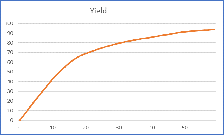 |
 |
A base is chosen and written into the matrix as a description of the unit’s operation and shift vectors are added to say how the changes when the parameter (or feed quality) moves away from that point. The base point and slope chosen influence where in the scope of potential values the LP will be most accurate. For example, 30 is taken at the base point and the delta yield from 29 to 30 gives the slope that is used to predict the yield at all other parameter values. . |
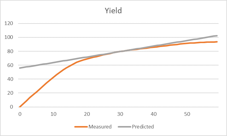
The predicted yield is very accurate in the middle, over-predicts a little at high values, and is very poor at low values. (Note that although I have labelled the original yield curve as “measured”, it is very unlikely that there is test run data over the whole range. You usually find that there is a concentration of actual data around the typical operating points and that this has been used to tune a process simulator so that values can be extrapolated to fill in the required range.) If the unit is unlikely to ever operate in the lowest conditions, then this large gap between measured and predicted is not important. Set a minimum limit on the parameter and avoid it. However, if the curve does cover the genuine range, then it will be very difficult to make a good representation with just a single base and delta
| One solution to this problem is to make a piece-wise linear representation. Create multiple copies of the unit (within a single set of sub-model tables or separated each into its own set) that cover different ranges of the key parameter value. Here I would make bases at 10, 30 and 50, each constrained to apply to +/- 10 units of the parameter. You can see from the individual lines that the slopes are quite different in each of these areas – and, most importantly, the gaps between predicted and measured yield are much smaller. | 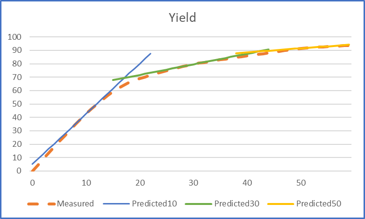 |
If you get a solution with just one base active, you have a more accurate prediction of the unit yield. But, since an optimization will take even the smallest advantage, you may find that solutions sometimes contain a mix of the different pieces. For example, it might split the feed between the first and last pieces instead of using the middle section, if the yield of a desirable material interpolated between those is higher than the stated one. For example, on the 30 base mode the yield is 79.6. But you can also achieve an average parameter of 30 by running half the feed on the 10 mode – using the shift vector to go up to 20 - and half on the 50 mode, shifting down to 40. The extrapolated yields are 71.7 and 88.5, giving an overall yield of 80.1. The model gets more of the good stuff than it should without breaking any of the rules.
How to stop the model from making that cheat? Put the Base modes in an SOS. In GRTMPS such sets are defined on a tab on the data node.
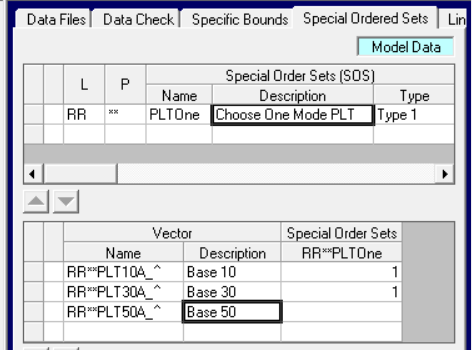
You have to list the matrix name of the unit operation, including any padding - that is (LL)(PP)(UNT)(OPQQ) -- , so check in the MTX, ROW or SPA files to be sure that you have the full name. (Although you can use ** as a wild card for locations or periods). Note that these set definitions are Model Data and so will be active in all the cases in the database. If you are using table-based input, the sets go in 196.0.
Sets are an extension of the traditional MPS matrix format so it is less standard between optimizers.
A matrix for H/CPLEX has
SOS
S1 .RRAAPLTOne
RRAAPLT10A_^ 1
RRAAPLT30A_^ 2
RRAAPLT50A_^ 3
While one for HXPRESS is
SETS
S1 .RRAAPLTOne
.RRAAPLTOne RRAAPLT10A_^ 1.0 RRAAPLT30A_^ 2.0
.RRAAPLTOne RRAAPLT50A_^ 3.0
HSLP does not support SOS.
If the name of a set members doesn’t match an active mode, it will be omitted. If your set doesn’t appear to be working, then chances are that you haven’t got the member names right, or that the location/period in the set name aren’t active. Any set which has fewer than 2 members is also not written out.
This piece-wise linear approach is rendered somewhat obsolete in GRTMPS by the Adherent Recursion technique. If you can express (or approximate) the non-linear relationship as a function, then you would usually be better off using AR to write a dynamic base-delta representation, so that the base mode and shift vectors are updated on each recursion pass. However, if you don’t have enough information for that, or if the curve is very awkward (has discontinuities or multiple inflection points), then piece-wise linear may still be useful (the pieces could even each be a PSI).
A word of warning, however, on mixing SOS and distributed recursion. The transfer of information about the difference between assumed and actual quality via distribution factors on error vectors is how the linear approximation has some understanding of the actual impact of quality changes. If a distribution is assumed to be zero, then the information flow is broken and the linear approximation will not contain any link between changes in feed qualities and the process operation. (This is why models often find better solutions when a small minimum is applied to the pool uses, as it keeps the connection active). With an SOS on the process modes, we have built-in a situation where distributions can only jump between extremes of 0 and 1 from one pass to another. Only the mode chosen on the previous recursion pass receives information about the quality change. A minimum distribution factors is unlikely to be helpful with a SOS as it may force multiple vectors to run for feasibility. Sometimes this distribution issue is not significant as the model may well immediately settle to the best option, but sometimes it will make the solutions oscillate so that the optimization does not converge.
What other applications are there for this in process industry planning models? I have seen it used for bi-directional pipelines, allowing inventory to move in or out of a tank but not both and alternative purchase or sales contracts. In distribution models it is often used for assigning a single supplier of all products to each customer – a nice little modelling problem that merits its own note.
From Kathy's Desk, 29th November 2023.
Comments and suggestions gratefully received via the usual e-mail addresses or here.
You may also use this form to ask to be added to the distribution list so that you are notified via e-mail when new articles are posted.