Planning models need to include all the options and obligations for your business so that it can find the best overall set of actions. Are there penalties for failing to fulfil contracts? Bonuses for exceeding requirements? While costs and revenues that are pro-rated to throughput or product quantities can be modelled with linear variables, contracts often include if… then clauses where the consequences – costs, revenues, capacity availability – come as a lump sum triggered by passing some threshold. For example, you might pay a penalty for not supplying sufficient product to a client (or putting enough throughput into a pipeline, or fail to satisfy a process sharing contract or to take delivery of a contracted feed material.) Or perhaps you have to pay a fee to secure the use of another tank or ship or terminal or train when the quantity of oil passing through exceeds the capacity of the current resource.
 |
The model needs to contain a representation of the rules, so it can balance the benefit of taking the action against the consequences of not doing so. If you have only a few such relationships you could handle them as separate cases – but if there are many such options, it will be more efficient to include them in a single optimization. If…then logic can be written for situations where an option can only be, or must be, active when a condition is met. These structures use integer variables and so turn the model into a MIP problem. There will be a binary variable that is usually set to on (1) when the condition is met and off (0) when it is not.
|
If…Then Logic Equations
Let’s start with a simple transportation example. The refinery that normally supplies a neighbouring region is going to be closed for a turnaround, so there is an opportunity to sell products there. It only costs $0.1/ton (or bbl or m3 as you use in your model) to move it there by rail, but you have to lease a train from the railway company. The leasing contract includes an up-front lump sum cost of $5,000/month that will need to be paid, regardless of how much is shipped, up to the maximum capacity of 1,000/tons per day.
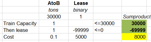
I always start the modelling for such rules by setting up the equations in Excel, to ensure that I have correctly captured the relationships. We need a binary variable that is 1 when the train is leased, but 0 when it is not. The capacity is available when the option is on, but can’t be used when it is off. For a monthly plan, we need something like:
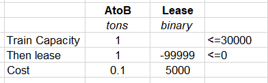
The variable AtoB represents the amount of product moved on the train. It is constrained to 30,000 (30 days hath September, April, June or November….). Note that the logic for such rules can be expressed in different ways. You can think of it as “If you pay for a lease, then you can use the train”, or “If you use the train, then you have to pay for a lease”. The latter perspective with the capacity always there, but not usable, is often easier to construct than generating the capacity when the variable is set, although that can, of course, be done. Lease is a binary variable that indicates if the lease has been purchased or not. If it is set to 1, then the 5,000 Cost will be paid in addition to the fee per ton.
The relationship between the tons moved and the lease activation is controlled by the “Then lease” equation. 1x AtoB tons – 99999 x Lease (0 or 1) <=0. The row must always be zero or negative. The -99999 is a “Big M”, a factor set to ensure that the equation can maintain a negative overall value when AtoB is positive but prevent any movement when Lease is 0. Let’s look at the four possible combinations of movement on/off and lease on/off to make sure they all do the right thing.
Scenario 1: No movement, no lease. Both variables are zero.
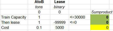
The constraints should all be feasible, and they are.
Scenario 2: No movement, but lease on.
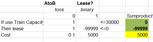
This is feasible, but uneconomic as it incurs a cost with no benefit so the optimization will naturally avoid it. You could block it explicitly with an added constraint 1 x AtoB – 1 x Lease >=0. Such a control forces a minimum movement if the option is activated and so is sometimes a useful addition with the coefficients adjusted to set the desired amount.
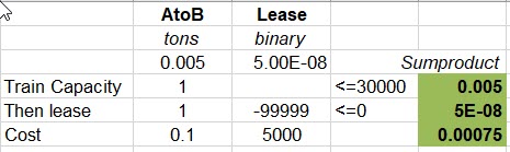
Scenario 3: Movement, but no lease. There is activity on the movement variable, but the lease is zero.
The “Then lease” row has a non-zero positive value so it is infeasible, as it should be.
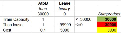
Scenario 4: Movement with lease. If there is a movement, then activating the lease should make it feasible.
Big M
You can see that there is a lot of slack on the “Then lease” row, so the Big M could be smaller, which would improve the scaling. The smallest value that works is the maximum on the movement – any smaller and you would be preventing it from reaching the maximum. However, this number usually ends up as a process unit co-efficient when set up in GRTMPS so it would have to be valid for all locations and periods, as well as actively maintained so that it didn’t accidentally become limiting. That could be done if you are using Table based input, but is not convenient in the database models. An arbitrary large value makes life simpler – but don't make it too big.
Very large Big M values are bad because they can result in apparent violations of your rules. (This is the very advanced bit.) You have to remember that mathematical optimization on a computer is governed by tolerances. The typical tolerance for feasibility in the commercial optimizers is 1E-6. So if the solution moved 30000.000001 tons it would be feasible (and you probably wouldn’t notice it). The binary variables are also subject to another tolerance that is often a little tighter – 1E-7 – for assessing if the value is 0 or 1. So 0.9999999 counts as 1, as does1.0000001 – while 0.0000001 is treated as zero. A solution is classified as integer if all the variables have acceptable values. This will often happen before the branch-and-bound has constrained them - very desirable for speed. When the Integer optimization finishes, a "FIXMIP" step is run by the optimizer that codes the best solution into the matrix by bounding the integer variables to 0 or 1. The problem should be immediately or almost so, optimal and replicate the reported best case objective value.
It is possible that the best solution contains some borderline feasible activities and constraints - such as this one – where the binary variable and the Then Lease constraints are not quite zero.
The "illegal" movement is very small and likely to round out of any reports, particularly when scaled to a per day value, if it is not knocked out during the FIXMIP optimization.
A larger Big M, however, creates more capacity on the edge of the feasibility tolerance. If I add a couple of nines to the co-efficient then
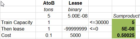
5 tons can be moved without buying the lease. If it makes it through the FIXMIP step you will be left with a wrong looking solution. Sometimes, the optimizer has to do some work to stay optimal when all the integer values are constrained and that might result in a different objective value, which is confusing. Sometimes, the problem will end up as infeasible which is annoying. The newer versions of H/XPRESS, at least, have some rather fancy logic to try to detect when something like this is happening and will dynamically adjust the tolerances and try again - something you can see in the optimizer log in the LST file.
Choose your Big M wisely!
If…then via GRTMPS
Now that we have a design, it’s time to implement it in GRTMPS. The easiest way to generate a binary vector is as a process unit operation. Movements are handled through the transportation panels, but can be connected to process limits so that we can make the “Then Lease” constraint.
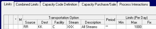
Here are the transport options that are being considered from refinery location RR to market location KK, via facility C, the train.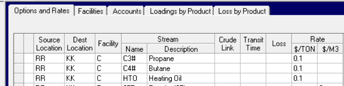
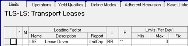
The maximum movement can be set on the transportation Limits – which are configured as daily values in this model.
Define a Loading Factor for the lease control and connect the transport options to it.
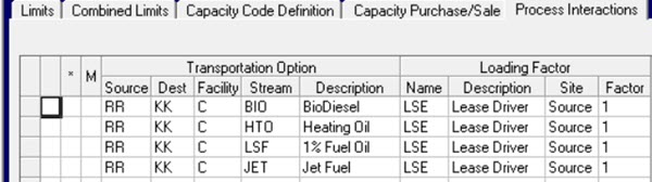
This panel is found on the Transportation Limits and Capacity sub-node. “Site” is a choice between Source and Destination and needs to match the location where the process limit will be set. I’m doing it at the refinery. (If you are working with tables, this information can be provided in either 801.5 or 141.4. They have somewhat different methods for listing the contributing options.) If there are different controls/leases for the different destinations then it might be more convenient to set the limits at the destination.
| You need a dummy process unit, active at the location where the factor is loaded (RR in this example). Define a mode to be your binary variable. On the Operations panel, right-click in the Bound cell to open the dialogue box and tick “Is MIP”. If you are working with Tables, use the $MIP column in 2xx.0. In newer versions of GRTMPS the presence of any integer type variables will trigger the MIP optimization – in older versions (pre 5.7) you have to activate it explicitly on the optimizer panel on the case node, otherwise the binary value requirement will be ignored. | 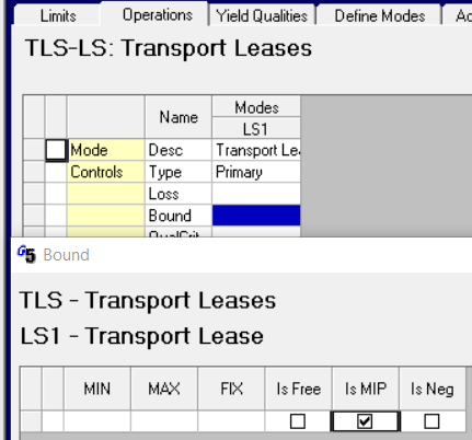 |
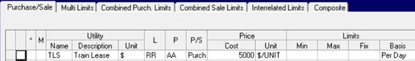
The price of the lease could be entered in the unit table on a Cost row – but I usually do them as utilities so I can then have different prices in different cases and/or at different locations and periods.
| The unit can now consume one lease and apply the Big M factor to the driver control. When setting up the unit operation, you have to take the RHS scaling into account. (Another advanced bit) This defaults to 1000 so for most models the 30,000 limit in the equation tests would appear in the matrix as just 30. Any bound or limit set to 1 would effectively be 1000. A limit of 1 would appear as 0.001. The binary variables have an upper bound of 1 because that is what the optimizers assign to that bound type - this makes it behave like a 1000 in the context of the scaled matrix, not 1. Since we can't change the scaling of the vector, we have to scale the contributors instead. So for 1 lease, we use 0.001. (If you have a model that is mostly integer variables and the limits are generally small numbers, set the RHS scaling to 1, so you don't have to worry about it.) | 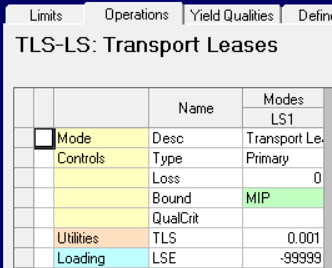 |
The lease driver is set to Max zero:
And then it is time to test what you are doing by pressing the LP button. The optimizer will turn the option on or off in order to maximize profit. It should be obvious from the economic and utility reports in an "On" solution if you have scaled things correctly If optimal the answer comes out as “Off”, you need to check that the structure is correct by forcing the model to use the option. In this case, a minimum on the movement or the sale at the destination can be used. It is also important to check that the model can choose “Off” even if the current economics indicate “On”. Block the option (e.g., no sales at the destination) to make sure that you haven’t unintentionally put in some minimum that keeps it always on. If any of the cases go infeasible, then use the Matrix Analyzer to check that your generated structure matches your design.
This example is quite simple but the structure can be extended to handle more complex situations. Perhaps this simple choice needs to be replicated to apply to a number of locations. Perhaps the “If” is a more complex condition -where more than one thing has to be TRUE before the THEN is triggered. Or you can have chains of logic. Sometimes Semi-continuous, Batch or Special Ordered Set structures can be used to avoid writing explicit controls -particularly if the decisions involve the activities of single vectors. Bear in mind there are always multiple, mathematically equivalent ways to express these things – and that MIP problems solve best when heavily constrained.
If this might be useful in your modelling, then I hope you are successful in implementing it.
revised 21st September 2022
You may also use this form to ask to be added to the distribution list so that you are notified via e-mail when new articles are posted.