Oil refinery and other process industry optimization problems are largely covered by Linear Programming models. Most variables represent continuous quantities, such as the amount of a component to mix into a blend, that are allowed to take on any real number value between a minimum and maximum. However, there are some constraints that are best handled with discrete variables. For example, the number of crudes purchased, rather than the total amount, can be restricted by using a set of binary variables, one for each crude, that is must be one if that crude is purchased but zero if it is not. A maximum on the sum of these variables will limit the number of crudes to be used. Semi-continuous bounds, where a variable can be zero or between a minimum and maximum, are also useful. Batch limits, where, for example, oil movements must be made in particular parcel sizes – 10,000 or 20,000, not 11,314.159, can make solutions more realistic. Some refinery models make use of Special Ordered Sets (SOS), where only 1 or 2 of the members can be active in the solution, to choose between different operating conditions on process units. A model that contains both linear and integer variables is an example of Mixed Integer Programming (MIP) and is traditionally solved using a Branch and Bound algorithm.
Suppose our matrix contained a binary variable for each of 25 crudes that could be bought. There would be 2^25 = 33,554,432 possible combinations. If we require a solution with between 1 and 5 crudes active there would still be 25*24*23*22*21= 6,375,600 combinations that might be feasible and probably many are. How to find the combination that produces the best value?
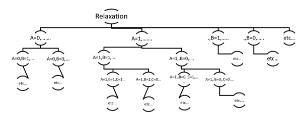
First, the “Relaxation” is optimized as if it were a pure LP and the discrete bounds don’t matter. The binary variables will be treated as having an upper bound of 1, but can take on fractional values. If this relaxed problem is infeasible (status INFE), there is no point in continuing, as enforcing more bounds will only make things worse. If the relaxation is optimal and it just so happens that all the binary variables have solved to 0 or 1 then optimization is already complete. It is more likely, however, that some of the binary variables will have fractional values so although the sum is within the maximum of 5 there are more active crudes than that. More work will need to be done to find the integer optimal solution.
Think of the problem as a tree whose branches divide when a binary variable is forced to be 1 or 0. Each combination is a node that has one more constraint than its predecessor.
The Branch and Bound method of searching this tree for the best possible solution is based on the fact that the objective value of an LP problem cannot be improved if constraints are added – (emphasis here on linear – that is a model that doesn’t use recursion, or the linear approximation from one recursion pass of an SLP model). The value of the relaxed solution, therefore, sets an initial upper limit, the Best Bound, on the objective value that could be achieved when the integer bounds are enforced. Once a bound makes the solution infeasible, it also can’t become optimal again by adding more constraints.
The B&B algorithm selects one of the binary variables to work on and fixes it to 0 or 1. This new problem can be optimized very, very quickly because the Simplex algorithm can use the basis – a list of which constraints are constraining – from the previous nearly identical problem to give it a head start. Suppose this variable, A, has been set to 1, so that this crude is active. All the other binary variables continue to be free to solve to any value between 0 and 1.
There are three possible outcomes: infeasible, integer optimal, optimal.
• If model became infeasible, then this branch of the optimization can be dropped. In fact, no further combinations in which A=1 need to be considered on any other branch.
• If the solution is integer optimal (sometimes referred to as a Global solution), the objective value becomes the Best Solution. This branch would be finished since fixing any of the other binary variables to a different value can only reduce the objective function.
• If the solution is optimal, but any of the other binary variables have unacceptable values, this node is still active.
For the next trial, the search has several options. If A=1 is still active, it could go down another level, keeping A=1, and adding a bound to another variable. Or it could switch to the other branch for this variable, A=0. Or it could move sideways and constrain one of the other variables to 0 or 1. (Optimizer developers have competed with each other for years trying to develop the most effective rules for deciding the search order.) Again, the optimization could be infeasible, integer optimal or just optimal.
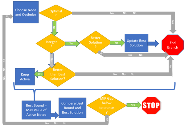
The Best Solution value will increase whenever a node solves to a better integer optimal solution than found so far. Only nodes with non-integer optimal solutions above the Best Solution value need to be explored further. MIP models benefit from having extra constraints, setting a minimum number of crudes for example, to help prune nodes out of the tree. The Best Bound will decrease as constraints are added. For example, once all the first level nodes have been evaluated, the maximum objective value of the ones that solved to non-integer optima will replace the value from the relaxation as the Best Bound. The difference between the Best Solution and the Best Bound is the MIP gap.
Here is the log of a branch and bound search by the H/Xpress optimizer. The Best Bound improves at 2 and 9, but an integer solution is not found until the 16th combination is tried.
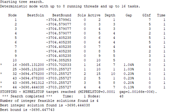
Three better solutions are found as the search continues. Solution and Bound come closer together and the gap drops. When the Bound and Solution become effectively the same, all the nodes have been evaluated or eliminated. In practice, as with recursion convergence testing, a tolerance is applied to this comparison. In GRTMPS the default MIP gap target is 0.01% of the Best Bound. This has been reached at the 48th node. Note that the solution was not improved after the 44th node; the remaining evaluations were just needed to reduce the Best Bound enough to be able to accept that 4th solution. Sometimes more time is needed to close the gap than to find the solution itself. With very large problems, the optimization may simply be terminated after a certain amount of time, taking the best solution found so far. If the relaxation was feasible but no optimal integer solutions are found, the status will return as MINF.
Recursion and MIP can be used together in GRTMPS, although combining the two presents some challenges. For example, recursion works best when connections are maintained between pools and their uses so that changes in quality effect the objective value - but integer solutions often include turning options off completely. If you are worried that the MIP structure is pushing an SLP model into a poor solution, remember that you can use multi-start to search for a better alternative. GRTMPS will still require the solution to be converged, not just integer optimal, so you can be sure it is still a feasible answer to the non-linear problem.
From Kathy's Desk, 12th November 2018.
Comments and suggestions gratefully received via the usual e-mail addresses or here.
You may also use this form to ask to be added to the distribution list so that you are notified via e-mail when new articles are posted.