Restrictions on refinery emissions are long established in many countries. Your planning models may already have a cap on SO2, or CO2 or flaring, so that production plans are optimized within the permitted boundaries. However, such a set-up is really asking the question "How much money can I make if I can maximize emissions?". There may be costs or credits associated with emissions and the economic impact of these will be taken into account, and may drive the model to reduce them. However, these costs are considered within the context of the overall profitability and may well be swamped by the benefits of maintaining high levels of utilization and production. Even if materials and processes with high emissions are only barely cheaper than cleaner ones, the optimization will select them.
If you want to explore the lowest possible emissions values, consistent with staying in profit, you need to configure the model specifically for that question. This is done by swapping the roles of money and emissions, such that the income is a constraint and the count of emissions is the objective function value that is minimized. In GRTMPS you can easily do this by applying the ALTOBJFN and MINOBJ options, as I will illustrate with a variation on the WT demo model. This model doesn’t have any explicit emissions tracking, but it seems reasonable to treat energy production from the burning of hydrocarbons as a proxy for them. Reduce the amount of energy utility produced and emissions will also drop.
Emissions Counting:
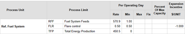
Although the alternative objective function can be any row in the matrix, it is usually most convenient to use a process limit, as you can apply loading factors to most activity types (purchases, sales, inventory, transportation, process operations and blending!). For the WT demo model, all of the energy required is produced on the Refinery Fuel Unit sub-model.
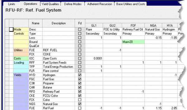
A blended refinery fuel oil (RFO), purchased natural gas (NGS) and a number of other streams are converted to Refinery Fuel (FUE as a stream in the Yields section), in proportion to their FOE (Fuel Oil Equivalent) energy value. This virtual stream is then converted to the FUE utility (operation GU2) to be consumed on the process units. Excess is disposed of to the Flare operation (GL1) in order to close the energy balance. (Think of it as waste heat or venting.). I have added a Total Energy Production (TFP) loading row to count the FOE produced - both converted to utility and wasted.
Emissions Constraint
In order to use Energy Production row as the alternative objective function, we need it in the matrix. The easiest way to add it is to put a limit on it.
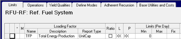
The objective function for the problem should include all the sites and all the time periods in the model, so the limit is set with XX for both the location and period codes.
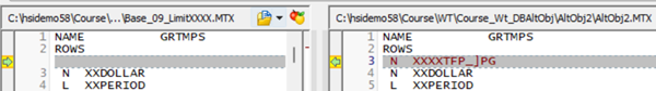
| Looking in the ROW file, I can see that when this is added to the matrix, the capacity code is padded with “_]P” to mark it as a process limit and finished with “G” for greater than. | Row = XXXXTFP_]PG Type = MIN RHS = 0.000000 RRAARFUGL1_^ = 1 RRAARFUGU2_^ = 1 |
Alternative Objective Function
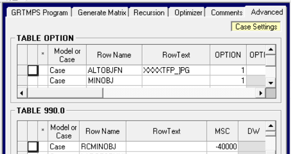
The full name of the row as it appears in the matrix is needed to set it as the Alternative Objective Function Value. This is done on the Advanced tab of the Case Data node, like so:
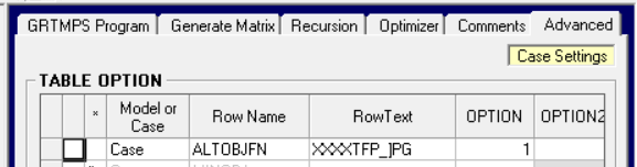
Note that this is a Case Setting so you can easily have a mix of cases with different objective functions within the same model database. It is only active if the 1 is present under column OPTION. (If you are working with table-based input data, you can either write this into TABLE OPTION as the database export does, or you can indicate the row in TABLE 111.0 using the column header $ALTOBJ. Be sure to mark only one row this way - and don’t use a limit with “**” as the period unless you are 100% never, ever, ever going to run a multi-period case.
The Matrix will now have a new “N” row
Some optimizers don’t allow more than one “N” row so the XXDOLLAR row might disappear. The RHS for the original constraint row will disappear so that it doesn’t matter what the Min limit value was.
Minimizing Emissions
The new objective function row has a big impact on the objective function value:
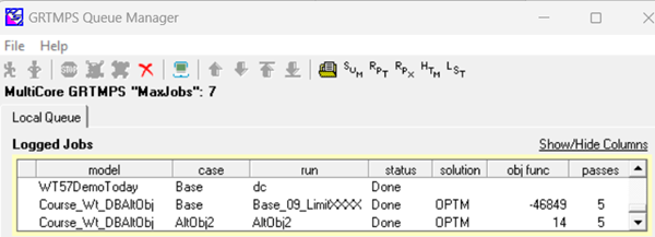
Instead of a gross income of
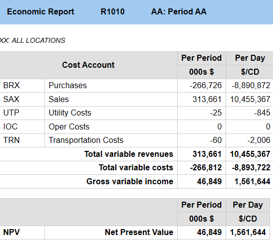
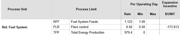
1,561,644 per day with an energy production of 979.4 FOE/day.
when the objective is to minimize Fuel consumption, gross income is
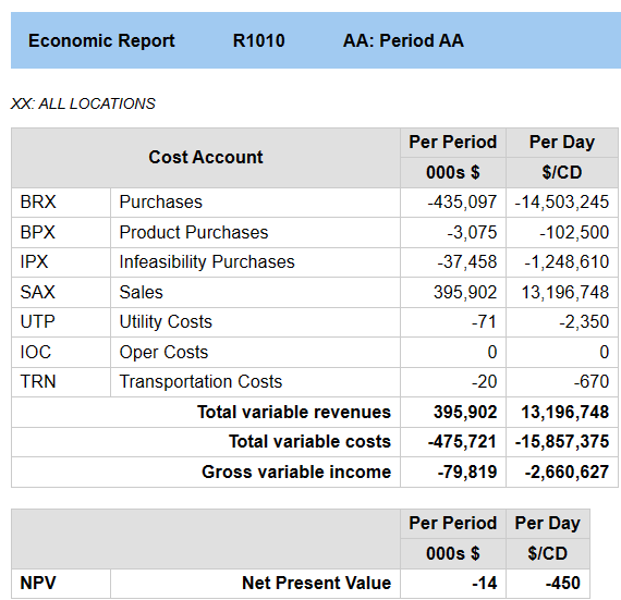
a loss of 2,660,627 per day, associated with an energy production of 450.5/day.
Note that the NPV (in the absence of a discount factor) on the Economic Summary is the value of the new objective function, matching the value shown for TFP on the Process Utilization report. The Cost Account section conveniently continues to show the usual sub-totals and income figures.
The energy production hasn’t gone all the way down to zero because the case has some product demands and minimum throughputs. If it didn’t, the best solution would be to turn everything off, as then there would be no energy consumption at all! The first time I ran this case, there was a lot of unused material as it made no sense to use any energy to process anything that didn't need to be sold, so I had to set all the streams to fixed balances and run it again. I left in the infeasibility purchases of hydrogen and the “buy not make” product purchase options in, so the model doesn't have to run the reformer and is satisfying some diesel demand externally. These actions do reduce on site emissions, but arguably there should be some count of energy used to produce and transport them. Whether to include those emissions in the minimization is a business decision and depends on the scope of the reduction you are studying.
Minimum Income
This plan certainly reduces emissions, but running at such a loss is not viable. We need a solution that preserves an acceptable level of income. This is where the Minimum Objective Function feature can be used to good effect. Considering the original solution total profit of 46,849 ‘000 $, I’m going to require a minimum of 40,000 (just because it’s a nice round number). Returning to the Advanced tab for the Case, I add the MINOBJ option and set the RCMINOBJ in the TABLE 990.0 grid (new with g5.8).
I have to remember to flip the sign so that it matches the raw optimizer output (as seen in the solution print and the queue manager).
The Gross Variable Income number in the Economic Report proves that the minimum target has been correctly set.
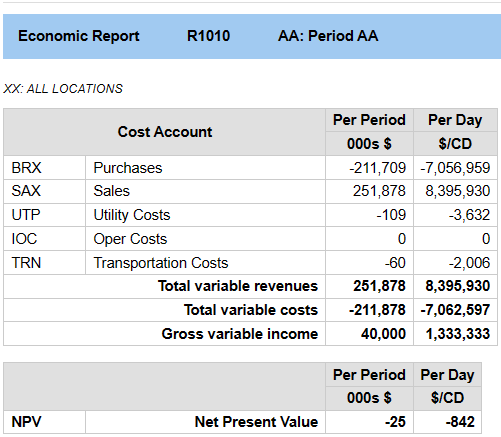
The NPV reveals that energy consumption has to increase to 842 FOE/day to achieve that income. This is considerably more than in the “who cares about money” case, but still an improvement on the 979 FOE/day emissions in the economic only optimization. Sacrificing $228,311/day, allows emissions to drop by 136 FOE /day (at the refinery’s current configuration) – or an average of $1,679/FOE.
Marginal Values
Did you notice how the marginal value on the minimum Flare (control FLR) changed from -173.19 to -1 when the alternative objective function was used? The limit is a minimum on the FOE that is generated but lost. A marginal value is the change in objective function for a unit change in the RHS of the equation. The original model is minimizing money, so the MV is $/FOE. When the objective function is itself FOE, then the MV is FOE/FOE and so must be 1. (Both are negative because it’s a minimum, and the benefit comes from being allowed to reduce the value further). You can use the marginal values to identify constraints that have the biggest impacts on energy consumption.
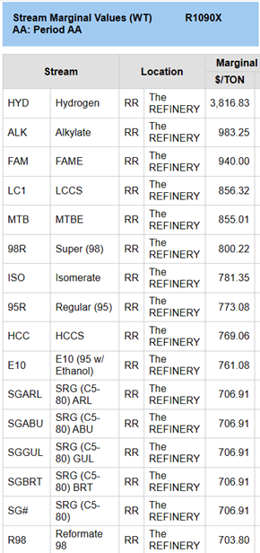
Stream marginal values also now in FOE/TON. Using this metric changes the relative values of the streams, as can be seen from the Marginal Value reports, ordered by value. The list on the left is the usual $/TON from the base case. The list on the right is from the FOE minimization case with the income constraint.
 |
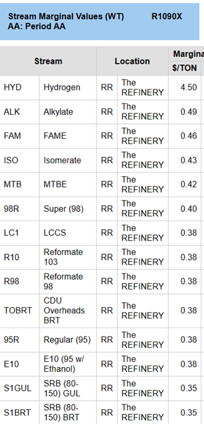 |
The FOE MV is interpreted in the same way as the $ one. That is, roughly, if you were given a ton of the stream for free, to do whatever you wanted with it, how much would that improve the objective value? So, if you had a free ton of either regular or E10 gasoline, it would save you 0.38 FOE. Considered from the energy requirement view, they have the same value – – even though one is sold for more than the other, so that their marginal dollar values are quite different.
.
There will also be a marginal value on the minimum value constraint. You can find it in the solution print.
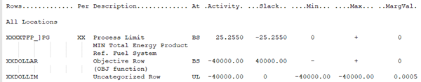
The XXDOLLIM row is a count of kilo-$ so the MV is 0.0005 FOE/$1000. Like all MVs, however, it is valid only over a certain range, and will change as other limits are encountered. To get a good picture of the relationship between the energy requirement and the money, run a series of cases at different target profit levels. The Case Generator tool will be useful for this.
If you are interested in this topic and have a tech support log in, you will also find a number of presentations from past user conferences by clients who are already making use of these features for emissions studies.
From Kathy's Desk, 11th October 2023.
Comments and suggestions gratefully received via the usual e-mail addresses or here.
You may also use this form to ask to be added to the distribution list so that you are notified via e-mail when new articles are posted.