The Matrix is the question and the Solution Print is the answer. The final result of an LP optimization is written out as a list of values for each variable and row, with its constraints and incentives. It is, of course, a mathematical view of the solution, which is why we all like to have output reports that translate it into a description of how the refinery (or whatever it is we are modelling) is actually running. However, it is very useful for debugging modelling problems, particularly infeasibilities and unboundedness. To prepare for some further work on those topics, here is a guide to reading the Solution Prints.
 |
I am taking my examples from the “Annotated Solution Print” that GRTMPS makes by adding descriptions so that it is easier for you to understand what the rows and columns do. (If you happen to spot something described as “Uncategorized” please let us know and will update the labelling code.) This is saved as the runid.SPA file, Output node, Other Output Files, when ANNSOL is included in the list of Extended Report segments. (Note that if the SPA is there but doesn’t contain all the rows and columns, then you have the Largest Marginal Value section active but not the Annotated Solution.) |
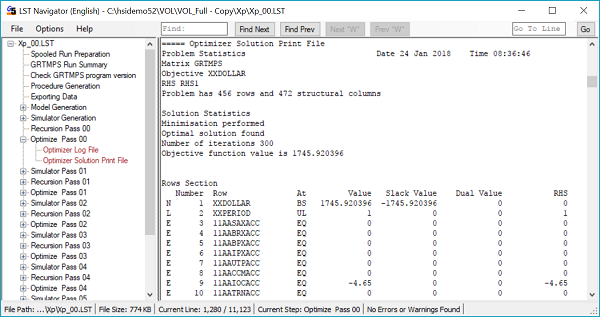
A solution print starts with a list of all the rows. Here is part of the rows section from the Time demo model.
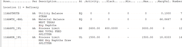
“At” tells you the status of the constraint. “Activity” is the sum-product of all the contributions to the row, its left-hand-side value. The “Slack” is the gap between the Activity and the limit’s right-hand-side (RHS).
BS under At is for Basic and indicates that the row is not constraining. The Marginal Value will be zero but the Slack will not. UL is for Upper Limit and indicates that the row is constrained to a maximum value. The Slack is zero but the Marginal Value probably isn’t. A minimum row hitting its constraint will be at LL, Lower Limit. Slacks for basic maximum limits are usually positive, while those for minimum limits are negative, although you could write rows where they take the opposite sign. If a row is at EQ it is a fixed constraint. In a feasible solution the Slack on such a row must be zero. The Min and Max are shown as the same for EQ rows; these are zero for the utility and stream balance rows shown, but are not necessarily so. If you have an infeasible solution, then any row with Activity that that does not meet its constraint will be At “**”.
The Marg.Val column displays the Dual Value, which is the incentive for relaxing a constraint. Number is just a counter for the rows. (I edited out some lines breaking the sequence.)
The columns section is very similar to the rows.
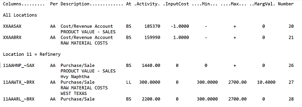
Vectors may have bounds at both ends, that are shown in the Min and Max columns. By default they have a minimum of zero, and a maximum of infinity, indicated here as “+”. Being At BS means that the variable is basic, active in the solution without being constrained by a bound. (Although sometimes the activity is zero, as if it is at the lower bound, but with no incentive). UL and LL indicate being at the upper or lower limit. If a vector has a negative activity in a feasible solution then it has been set FREE, or explicitly given a negative lower bound. At EQ indicates a variable fixed to a specific value, min = max. “**” indicates an infeasible Activity. The marking of an unbounded vector (one that contributes value but has no constraint to stop it reading infinity) varies with optimizer. H/XPRESS shows it as At “++”; HSLP uses ++ in the LST file, but ** in the Annotated solution. H/CPLEX does no use the At status to indicate unboundedness.
Input Cost shows the intersection between the variable and objective function row. Because GRTMPS matrices are written with the prices collected into separate rows for each Cost account (CLASS OBJ), only the vectors, such as XXAASAX in the example, that transfer the sub-totals into the objective function have any connection. This is usually +1 for costs and -1 for revenue as we write minimization problems. The Marginal Value column shows the Reduced Cost, the incentive, for variables at a bound.
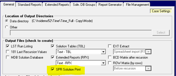
The solution prints written directly by the optimizers show the same information in a similar format. They are without the helpful notes on names, but more compact as a result. You can usually find a solution print in the LST file. This is controlled via the Optimizer, Advanced settings on the Case nodes.
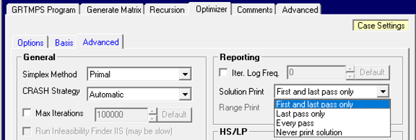
The default option is to include the prints for the first as well as the final solution, so this can be helpful in understanding what is happening as your model is getting started. You may reduce this to the Last Pass Only (TABLE OPTIMIZE, NOPRINT = 1). Including the solution print on Every Pass (TABLE OPTIMIZE, RCPRINT=1) can be helpful in diagnosing mid-run infeasibilities, but will make for a very long LST file and so is not something you would want to leave on. When running a non-recursed model, the solution print will be included in the LST file unless the Never option is chosen. Within the LST file the solution prints can be conveniently found in the Optimizer steps, using the LST Navigator. Note #16 Decoding Matrix Row and Column Names can help you translate the row and column names.
You can also direct a copy of the last pass solution print to the file runid.SPA, unless you have chosen “Never Print Solution”. Mark it as Keep on the General Output panel.
From Kathy's Hotel Room, Neustadt a.d. Donau, 24th January 2018.
Comments and suggestions gratefully received via the usual e-mail addresses or here.
You may also use this form to ask to be added to the distribution list so that you are notified via e-mail when new articles are posted.