92) Batch Limits

LPs will set an optimal activity to about 15 decimal places (if you look at the solution print rather than the report where things are always rounded), so you may find solutions that buy, sell or move amounts like 31,415.92653589 m3. (If you don’t hit a limit.) You aren’t going to give operating instructions to such a precision. Furthermore, if the feedstock or product is delivered by ship, barge, truck or train cars, then it is likely that you aren’t going to send or receive one that is close to empty.  That is if you can put 5,000 m3 in each shipment, you are unlikely to send out the 7th one with just 1,415 in it.

For long range and mid-term planning purposes, this sort of detail can probably be ignored.  The answers are good enough, given all the other assumptions you have to make. Any “remainders” can be regarded as something that just rolls forward. But if you are trying to do near term planning, perhaps in tandem with operational scheduling, or have a distribution model that takes your disposals to a more detailed breakdown (in terms of what is sent to each client, rather than the total that leaves the production facilities), then perhaps the discrepancies between LP solution values and practical options are enough to make it matter. Is the solution still feasible if it has to fit into discrete delivery batches? Would you be better off rounding up or down?

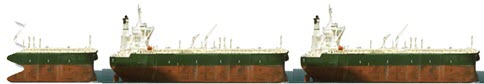Another area where batch limits can also be useful is crude purchases, particularly for a refinery where some grades come on very large ships. In many LP models, crude purchases are set up just to provide the material that is processed – that is they assume complete flexibility to consume any amount – but this is different from what you can buy.

By definition, variables in LP models are continuous. You can give a minimum and a maximum bound on an option – but the solution can take any value in between. To constrain the solution to only use discrete values that are multiples of the allowed cargo sizes, Mixed Integer Programming (MIP) must be used.   GRTMPS has a feature to set this up for you automatically for purchases, sales and transportation limits. For example, Exercise 22 in the Wt Demo model applies a batch limit to one of the crude purchases, like so:

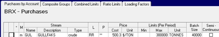
The number in the Batch Size column is always treated as a total amount; it is not multiplied by period duration, even if the purchase account is configured for daily limits. However, it should be given with the same scaling as the regular limits. Here they are all in tonnes, but if the model was configured for limits are in kilo-tonnes, then the batch size must be too. That is, if the max were expressed as 300 kt, then the batch would be 40 kt.

Equations for Batch Limits
Batch constraints are built using a Lower Integer (LI) bound of zero, written like this in an MPS format matrix

BOUNDS
   LI   BOUND1  RRAAGUL_~BRI   0.0

The variable can only have a positive integer value in the solution: 0, 1, 2, 3, 4 etc. This discrete variable is used to indicate how many batches are taken. It must be linked to the variable that represents the option to be controlled such that the number of batches is multiplied by the parcel size to give the total amount.   Putting the answer to Exer 22 into the Matrix Analyzer shows how this works. 

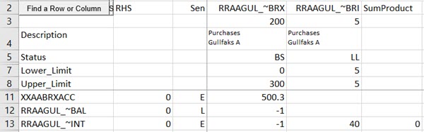
The “INT” limit makes the link. Note that the default RHS scaling used in this model makes the batch size co-efficient scale down to 40, while the maximum is the Upper_Limit of 300.
The solution uses 5 parcels of this crude.  (This is rounding up compared to the base case solution; Rounding down must have resulted in a lower objective value.)  Although the integer variable RRAAGUL_~BRI started with the LI 0 bound – as would be visible in the matrix file -  in the Solution Print  it is reported with both Upper and Lower limits of 5. This is because the best solution from the integer optimization finished with a “FIXMIP” step.  The discrete variables are constrained to their optimal values, then the problem is solved again in order to obtain a full basic solution with incentives.

It isn’t necessary to have a maximum bound on the purchase to make this work (unlike a semi-continuous bound), but MIP models solve better with more constraints. The maximum on the purchase will make any solution that takes 8 or more batches infeasible.  The MIP algorithms can use that implication to make better branching choices and reduce the number of nodes that are searched.

Batch Limits and Incentives
The batch limit has an impact on the marginal economics for the crude.

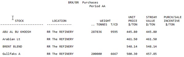
The marginal value of Gullfaks is LESS than the price (500.3 as you can see it in the Matrix Analyzer screenshot), indicating that it has had to buy MORE of this crude than it would like.  The absence of an incentive indicates that this is not due to a minimum bound on the purchase vector itself, but because some other indirect constraint prevents it from reducing the amount. 

With a batch limit, we know that constraint is the INT row. Go back to the Matrix Analyzer and expand the row details:

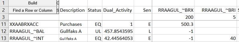
The Internal INT row has a Dual Activity (a.k.a. Marginal Value) of 42.44. This is the difference between the price and the stream marginal value. Note that this value corresponds to relaxing the RHS from 0 to 1, with all other things being equal. It is how much the objective value would change for this linearization, if you were allowed to buy 199,999 tons. It is not the value of the last parcel, or the batch size – but rather what would be gained if the last parcel was one ton less than it is.

Balancing out the Material Balance
If you use batch limits – particularly for large amounts such as the crude deliveries, but even also for numerous small product deliveries - you need to think about how to handle an imbalance between the processing/production amounts and the batch multiples. The refinery or your distribution network probably doesn’t need to operate as if it was restricted to exact multiples of the batch amounts within any specific time frame because there will almost certainly be storage or other options to smooth things out.  The model, however, will behave as if that is a strict requirement unless you give it some means of balancing out the amounts.  Often this is done by allowing the model to send excess material to inventory.  You can do that even with a single period model. The impact of allowing closing inventory or some other alternative disposal will depend on the value assigned to that material - the crude that isn't processed or the product that isn't sold. 

I set up four additional cases with inventory as an option for the Gullfaks A crude, giving the closing inventory a value that was: Just Below the Marginal Value; Just Above the Marginal Value; Midway between MV and Price; the Price – and then adapted one of the Report Generator MC Templates (with a bit of further editing after generating it to make it more compact since I was only doing this once) to compare the relevant KPIs: Crude Purchased, Crude to Inventory and Marginal Value.

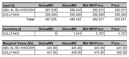
When the closing inventory value is less than the marginal value from the original “to buy is to process case”, nothing is sent to inventory. What would be the point?  Once the inventory value is more than the original MV, then material will start to move to storage.  The processing capacity that is made available by diverting the Gullfaks is taken up by the ABU crude, although not one-to-one by ton. Note that even as the quantity is changing, the marginal value of ABU remains equal to its price. There is no limit on the purchase, so the LP solution will always balance at that point. The MV of GUL is different in each case, however. As the MV is the price of the next best option, it becomes the inventory value as soon as that exceeds the original MV, which reflected the gross product worth of the crude.  Thus, we can see that the value assigned to the crude that is not processed has a significant impact on the solution and the apparent economics and so must be approached with some consideration as to your views on holding costs, etc. There is no easy answer to what this price should be.

A way of reducing the impact of final inventory valuation is to extend the time horizon of the plan by adding periods so that there is an opportunity to process any crude that was not needed in the first planning period.  The model can then optimize in response to its intrinsic value in line with your price forecasts.  You could also consider applying the batch limits in the first few periods – finishing with one or more periods where continuous amounts can be bought or sold.   The rationale for that is that as there is certainly increasing uncertainty in pricing and demands as you look further ahead, solutions for more distant months are providing guidance rather than plans. The more logistical constraints could be considered only when the planning period in question is within the horizon where the purchases/sales would need to be made.  However, there will of course be a trade off against speed and stability as the model becomes larger and more complex, so you may need to experiment with different combinations to find the number of periods and the degree of constraint that gives you enough detail to make a good plan without making the model difficult to manage