What do cleaning a fish, climbing a mountain peak, and LP models have in common? They go better if you are good at scaling!
Scaling in LP models is about the range of magnitude of values that appear in the equations. If you have a mix of very small and very large numbers it makes it harder for the optimizer to solve the problem. This is less of an issue with the 64-bit precision calculations that are now used, but it is still often the case that an optimization step that is taking an unusually long time will be issuing complaints about bad scaling. You can improve the scaling of the model in local ways by deciding what units to track properties and utilities in and how you write process operations.
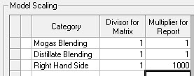
If you are working with GRTMPS there are also some overall Model Scaling factors. These are entered on the Model node and translate into TABLE 990.0 If a value is not given, defaults are assumed, so for some models this grid is empty. If the defaults were filled in, it would look like this:
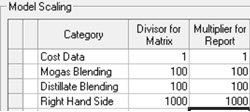 |
or | 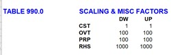 |
with the rows in the same order. ( I have no idea why the mogas one is tagged as “OVT” – we are into deep geological coding time with this feature.)
The scaling factors are normally given as powers of 10 so that applying them moves the decimal point. Inputted numbers are divided by the Divisor (DW) as they go into the equations, and the related results are multiplied by their Multiplier (UP) when retrieved from the solution.
I couldn’t find a model where the Cost scaling had been changed, so I think the default is fine (maybe if you had a model in a currency subject to hyper-inflation?). For models with non-linear process units (PSI or AR) or non-linear blending, it is better to set both Blending values to 1 as I have done below in the asymmetrical scaling example. The RHS factor of 1000 is still a reasonable value, but other factors are used as well. So I’m going to focus on that one for now, and leave an explanation for my blending recommendation for another time.
RHS Scaling
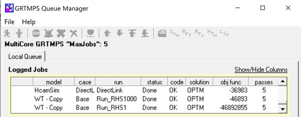
The RHS factors apply to unit capacities and all the other min/max/fix quantity limits on purchases, sales, inventory, transport, blending etc. (They are applied to BOUNDS as well but have no effect on ratio controls). 1000 is usually a good RHS scaling factor for models that are used for monthly or quarterly planning. By default GRTMPS writes optimization problems in terms of the total capacity available in the time period given. (Although there are other options). If you have a process unit with a maximum capacity of 25,000 m3/day (or tons or BBLs), and set up a case for February, the total capacity available is 725,000. (2020 is a leap year). Process operations are usually written in terms of 1 unit of feed, so the capacity equation, unscaled, would probably be Σ(1 * operation) <= 725,000 m3 The scaling of any individual row is the largest of any of the co-efficients and the RHS, divided by the smallest. So this row has a scaling of 725000/1. Apply the RHS scaling factor of 1000 however, and the equation becomes Σ(1 * operation) <= 725 km3. Scaling reduced to 725.
The RHS factors apply to unit capacities and all the other min/max/fix quantity limits on purchases, sales, inventory, transport, blending etc. (They are applied to BOUNDS as well but have no effect on ratio controls). 1000 is usually a good RHS scaling factor for models that are used for monthly or quarterly planning. By default GRTMPS writes optimization problems in terms of the total capacity available in the time period given. (Although there are other options). If you have a process unit with a maximum capacity of 25,000 m3/day (or tons or BBLs), and set up a case for February, the total capacity available is 725,000. (2020 is a leap year). Process operations are usually written in terms of 1 unit of feed, so the capacity equation, unscaled, would probably be Σ(1 * operation) <= 725,000 m3 The scaling of any individual row is the largest of any of the co-efficients and the RHS, divided by the smallest. So this row has a scaling of 725000/1. Apply the RHS scaling factor of 1000 however, and the equation becomes Σ(1 * operation) <= 725 km3. Scaling reduced to 725.
If you are setting up a case for 1 day or for a very large amount of time or total capacity, then you could try a different factor. You will see that the magnitude of the objective value will change in step with the scaling factor. The application of the UP factor in the RHS1000 case will bring it back to the same value as the RHS1 case in the results. (Although the economic reports are often set to show ‘000s $ - another scaling choice).
If the up and down factors are the same, for most models changing the RHS scaling does not require you to make any other adjustments. Very occasionally, perhaps if there is some intricate rule implemented with MIP structures, there are co-efficients in the process units that need to be in the same magnitude as the process limits. If you have one and miss it, you may get quite a different answer when you change the scaling factor. However, even when models are mathematically equivalent – the same except for the magnitude - they won’t necessarily converge to such similar answers as the demo model does. The differences in precision that result from changing the magnitude are very small, but even small differences can send models on different recursion paths. (which does make changing the scaling a means of assessing stability).
Input Scaling
A scaling factor can also be given for limits entered for the categories of data that have been marked as on a “per Period” basis.
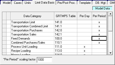
For purchase and sales the day or period choice is made on the Cost Accounts panel. If you are using table input, the scaling factor goes in TABLE 199.0 along with the list of tables that will have period data. With a factor of 1000, a minimum sale of “2” is actually 2000. (Ignore the labels a bit, please, you could change it to say KM3 – but then the report headers come out a bit funny for other types of data. This will be done better in g6.).
This scaling, however, does NOT affect the matrix. The input number is translated back to model units first. The 2 is read as 2000 and then the RHS scaling factor is applied. If that is also 1000, then the bound will be back to 2 as input.
Asymmetrical RHS Scaling
| Another way of scaling the input data is to use asymmetrical factors. This method moves the decimal place for all limits, whether given as per period or per day values . With a Divisor (DW) of 1, the limits will be written as inputted. The Multiplier (UP) of 1000 though, indicates that they are actually kilo-units. With this set up your 25,000 m3/day of capacity would be entered as 25. Multiplied by the 29 days of February it would go into the matrix as 725. So you end up with the same equation as when the larger value was input and then divided by 1000. |
 |
If you are using asymmetrical factors, the Period scaling factor should be 1. Remember that 2 is read as 2000 if the period factor is 1000. Dividing down by this RHS of 1 into the matrix, would leave the bound at 2000. Multiplying back by the 1000 Up factor after solving, and you’ve got 2,000,000 – probably not what you wanted.
If you are using asymmetrical factors, you will have to do more work if you want to try a different magnitude. The input data relates to a certain ratio of DW/UP. If you change that you need to move the decimal places on the inputted min/max/fix numbers.
Corporate Models
If you are combining models into a multi-location corporate model, the sub-models all need to work with the same DW/UP ratio (and the same "per period" factor, if that is used.) These Scaling factors are model level settings so the same value (the last one read) will be used for all data. It doesn’t matter if one model used 1/1 and another used 1000/1000. You should be able to run the pair under either setting. However if one model is 1/1000 and another is 1000/1000 when you put them together you will need to decide which one to use and update the other one’s data accordingly.
Time to go check your scaling factors and see what impact a change might have. I haven't done a systematic study of the impact of RHS scaling on the recursion behaviour, as I have largely set factors with a view to working with conveniently sized numbers. You might find a higher peak (unless its all just a red herring!)
From Kathy's Desk, which has left the EU without moving
19th February 2020.
19th February 2020.
Comments and suggestions gratefully received via the usual e-mail addresses or here.
You may also use this form to ask to be added to the distribution list so that you are notified via e-mail when new articles are posted.
You may also use this form to ask to be added to the distribution list so that you are notified via e-mail when new articles are posted.