Systematically varying an operating parameter such as severity is a fairly common task for the user of a refinery planning model. We do this when we are building models to check that the unit representation – whether non-linear or simply delta-base or modal -- works well over the whole of the expected range and is appropriately sensitive to changing conditions. As a part of our planning practicies going forward it is a means of gaining an understanding of the economic impacts of a parameter as well as a chance to study how the overall system adapts as it changes.
Suppose, for example, that you have a process unit in your refinery model that has a “severity” parameter – a reformer perhaps. The more severe the operation the better the quality, but the higher the energy costs, and the lower the throughput and yield – up to a point (as yield can't go negative for example). Planning cases would normally be run with the severity open within the possible (or typical range) in order to determine the optimal value (under the given assumptions). If the solution ends up at either the minimum or maximum you will have a marginal value to give some indication of the economic impact. However, if solves to an intermediate level then the marginal value is zero – not because severity is unimportant, but simply because it is not directly constrained. Any move away from that optimal point will reduce profitability.
To gain some understanding of the magnitude of the impacts of this operating condition as well as confirming that the model works will over the whole range, you should try varying it systematically. The best way to set up such a series of cases in GRTMPS is to use the Case Generator, which can be opened via the Tools menu in the g5 user interface. You need a base case to start from and if you put your cursor on the output section for that run, then it will be selected automatically when Case Gen opens. If not, you can use the GRTMPS model button or just browse (the button with 3-dots next to the name), to select your base run.
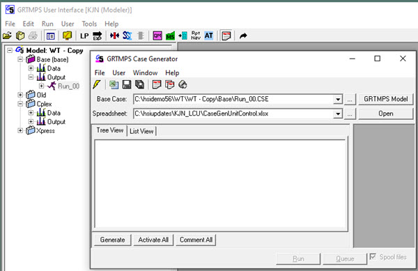
The scenarios are set-up in the "Spreadsheet". With a bit of thought this can be done in a way that is relatively generic and easy to configure to handle multiple situations without a lot of editing. You can change almost everything about your model in these cases – provided that you know the input table for it. (Sorry database input users, but from release 5.6 Beta 1.2 in August 2020 there is a new format for some types of data, including process limits and purchases/sales, that looks more like an SSI). Process operating parameters and capacity limits are almost always in TABLE 111.0 (1).
Within the case generator work book, each case is started with a header row, which gives it a name and defines how the data is to be used, followed by the data itself. Here is a screen shot of my general “vary a process unit limit” case generator spreadsheet that I use for testing models. It is set up to vary the reformer severity in the WT demo model.
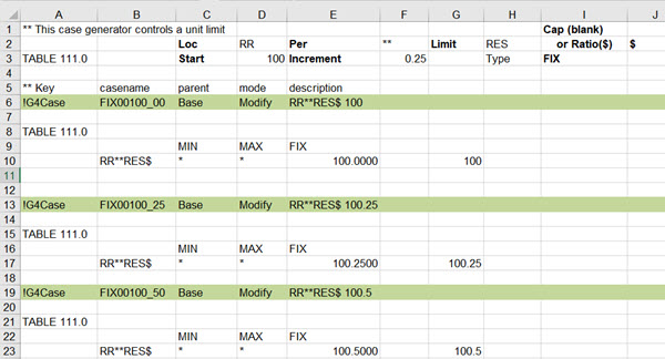
The header row for the first case is labelled by way of documentation. For this sensitivity task Key will be “!G4Case” (even if you are running g5.) . The case name will be appended to the base run name. It must NOT have any spaces or delimiter characters (such as “.” or “,”) in it. For this set of cases the parent is always “Base” – that is each variation is applied to the original run. Mode is always “Modify” because we are changing the data for one limit, not replacing the whole of the limit set. Finally, we have a description to remind us what the case is. (This is, of course, all explained in more detail in the Case Generator Help file).
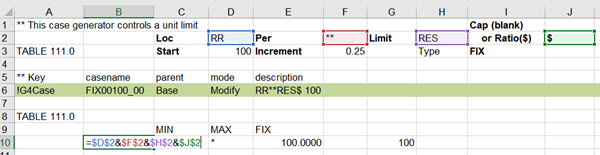
Each of my cases changes one process limit constraint by putting a value under MIN, MAX or FIX for the corresponding row in TABLE 111.0. Because I want to be able to use this for any model without messing about editing the cases, I have used formulae to create the case name and description, configure the row name, choose the column, and set the value. The refinery in the WT demo model uses location RR so that goes in cell D2. Same limit to apply to any period, so "**" in F2. The severity control is RES and it is a ratio, so $ in J2. (For a unit capacity limit, J2 is blank)
The row name in TABLE 111.0 is the same for every case: location-code + period-code + limit code + suffix – made by concatenating the entries in the top section, before the first case.
The parameter value sequence is calculated from the Start value (D3) and Increment (F3). The first case uses the start value. Subsequent cases use the previous case plus the increment. You can count down by using a negative increment. The type of constraint is set by entering MIN, MAX or FIX in J3. For this kind of operating parameter study I would normally set it to a FIX value, (although converting that to a narrow MIN/MAX to give it some wiggle room and get a marginal value if its an input to a non-linear unit model might be smarter with a more complex model). To avoid any conflict with a limit already in the model, the limits which are not being used are set to “*”, which wipes out any base case values.
The case name is the tricky bit. I could have just numbered them, but I do really like to have something that tells me what the run is. I started off trying to simply combine the constraint type with the value – BUT that doesn’t produce a valid name if the number is not an integer. After some tinkering about, I figured out how to convert the value to text, replacing the decimal separator with an underscore.

When your spreadsheet is all set up, go back to the Case Generator interface and press the “Generate” button (bottom left)
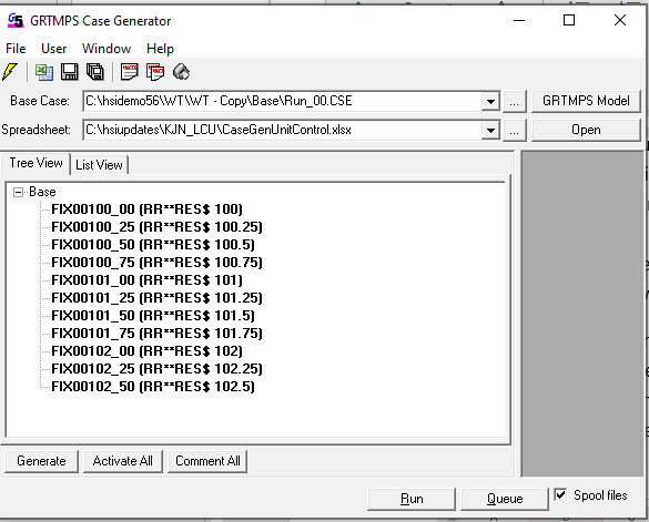
Then press the Run button to send them off. Make sure the Spool Files box is ticked if you have multi-core so you run more than one at a time and finish sooner. You can see I have 11 cases set up – if I want more, I just need to copy the last case section and paste it below. If I space it correctly, the formulae will take care of the value and name, etc If there are too many, you can comment cases.
When the runs are finished you can use one of the reporting tools to have a look at the results. I’ve used the MC_Economics template from Report Generator, and added a graph.
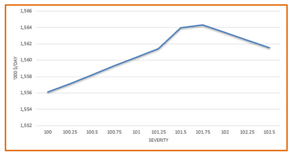
All the cases converged to optimal solutions, so this range is well covered by the model. (There is a reason I started at 100 and not 90.) The base case solved to 101.7, so the peak at 101.75 is as expected amongst the values tried, with a decline on either side. This is indicating a relatively simple relationship between severity and value, although not entirely linear as the slope does change as we move along.
However, more complex models might not be as well behaved. You might, for example, see more than one peak
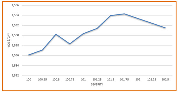
Your initial reaction is quite likely to be that the case where the dip occurs, 100.75, has solved to a poor value local optimum. That is possible and can be tested for by doing multi-starts to look for a better solution. However, you should also bear in mind that the relationship between a parameter and profit is not necessarily smooth. It may well be that there is more than one useful strategy. Perhaps, for example, this secondary peak occurs because there is a point where the higher throughput and lower costs compensate for the reduced quality. This benefit can be lost as costs rise and yields drop – but then, eventually, all the downsides of higher severity are overcome by the benefit of the improved quality. A simply linear, convex model would always find the highest peak, but the non-linear SLP type models (with pools etc.) that are usually used in the refining industry might get stuck on the weaker strategy. If that is found first during the recursion iterations it might converge there as everywhere else in the immediate vicinity looks worse. This is another good reason to study the sensitivity of the model to operating parameters. If you are aware of situations like this you can check which strategy the model is finding when left to optimize and give it a nudge in the right direction if needed.
Ready to have a go? As a starting point, there is a version of my Generic Parameter Case Generator workbook included with the Wt Demo model from v5.5 SP1 onwards – if you are running something older or want my latest enhancements, just e-mail tech support and I will be happy to send you a copy.
From Kathy's Desk, 25th October 2019.
(1) The exceptions are unscaled limits which are in 111.1. Process limits can also be given in 2xx.1 although in most table based models this is used for limits that are part of the unit structure and so shouldn't be changed, ever. In the database limits with constraints on location ** are exported to the unit table. If this is something that you do want to vary then the easiest approach is to set the location to a specific code instead so they come out in TABLE 111.0.
Comments and suggestions gratefully received via the usual e-mail addresses or here.
You may also use this form to ask to be added to the distribution list so that you are notified via e-mail when new articles are posted.
You may also use this form to ask to be added to the distribution list so that you are notified via e-mail when new articles are posted.