It is very useful for the refinery industry that many of the stream qualities that we need to predict – for product specifications or to ensure suitable unit feeds – blend linearly. Density scaling might be needed if the property blend basis is different from the model material balance basis (for example, sulphur in a volume model or benzene % volume in a weight model) as I described in my earlier note on linear blending (#44). However, there are often further complications. What if the property of the final blend is not simply a linear average of the component contributions?
Vapour pressure, octane, cloud point and viscosity are examples of properties where a simple proportional average of the measured values of the components will not tell you what value a mixture will have. Many of these are properties that don’t correspond in any simple way (that is currently known) to a measurable chemical characteristic of the material. Sometimes the original measurement tests were analogue (octane in an engine for example) so it is not surprising that they don’t behave neatly. So, how are we to optimize blends in our LP / SLP models and be sure that the recipes in our solutions result in on-spec products in practice?
Vapour pressure, octane, cloud point and viscosity are examples of properties where a simple proportional average of the measured values of the components will not tell you what value a mixture will have. Many of these are properties that don’t correspond in any simple way (that is currently known) to a measurable chemical characteristic of the material. Sometimes the original measurement tests were analogue (octane in an engine for example) so it is not surprising that they don’t behave neatly. So, how are we to optimize blends in our LP / SLP models and be sure that the recipes in our solutions result in on-spec products in practice?
Many such properties can be handled linearly after all, if a blending index is applied. An index is a formula that transforms the measured component properties into some other numbers which when averaged together give you the index value of the mixture. These are often log or power functions such that values at the far ends of the scale have considerably different impacts on the combined value. The blend value can then be found by inverting the formula to return the corresponding quality. (There are also indices that have been developed to blend to property, rather than index to save the final conversion – a useful attribute in pre-calculator days, but rather rare.)
For example, the Refutas index for viscosity applies the formula
14.543 x LN(LN(cSt+0.8) + 10.975
to kinematic viscosity measured in centistokes (cSt) at any temperature.
How do we use this? Suppose that you are making a low sulphur fuel oil with a requirement of a viscosity at 100 deg. C of 30 cSt. Your base heavy oil pool is at 34 cSt so you need to add a lighter material as a diluent to bring it on spec. If that stream has a viscosity of 1.5 cSt, what is the minimum needed in each ton of product?
| First, convert the component values and the specifcation to index | cSt | 34 | 1.5 | 30 |
| VBI | 29.389 | 8.318 | 28.880 |
Let x be the weight fraction of diluent needed. As we are blending just 1 ton, the base oil fraction will then be 1-x.
29.389 (1-x) + 8.318 x = 28.880
29.389 – 29.389x + 8.318x = 28.880
-21.071x= -0.509
x=0.0242
29.389 – 29.389x + 8.318x = 28.880
-21.071x= -0.509
x=0.0242
So your mixture should be, roughly, 2.4% diluent by weight and 97.6% heavy oil.
If you had done a linear blend without converting the values (an exercise left to the reader) the solution would be 12.3% diluent, an order of magnitude different. (The index in this case, had the effect of increasing the impact of the low viscosity stream.) If you used that much diluent, applying the index, the predicted viscosity is:
0.123 x 8.318 + 0.877 x 29.389 = 26.8 VBI, that is 19 cSt
by the index to quality formula: exp(exp((VBI - 10.975)/ 14.543))-0.8
If the index is a indeed a better predictor, then you would have blended to a large giveaway. Is the Refutas index blending a better predictor of product viscosity? In this case, almost certainly yes. This is an established method that is widely used. Is it the most accurate method? That is hard to tell. There are other viscosity indices and one of them might work better for your blends. If you are working with very light streams, you will definitely need to do something else, as the formula only works for values greater than 0.8 cSt.
There are also many indices to choose from for other properties – such as RVP, cloud, flash, pour point etc. Many oil majors developed their own, driven in no small part by the desire to be able to generate blend recipes in their LP models. These are valuable intellectual property and often treated as confidential. (When I started at BP in the 1980s the books of indices were numbered and registered to a particular holder, needing to be produced at an annual audit). There are also many available in the public domain. If you are a Haverly client, you have access to the HSI UDF Toolbox as an Excel add-in (UDF = User Defined Function) which has been put together by Kirby English. Amongst other things, this contains examples and documentation for a large number of blend indices. Here is the help entry for the Refutas index calcultion.
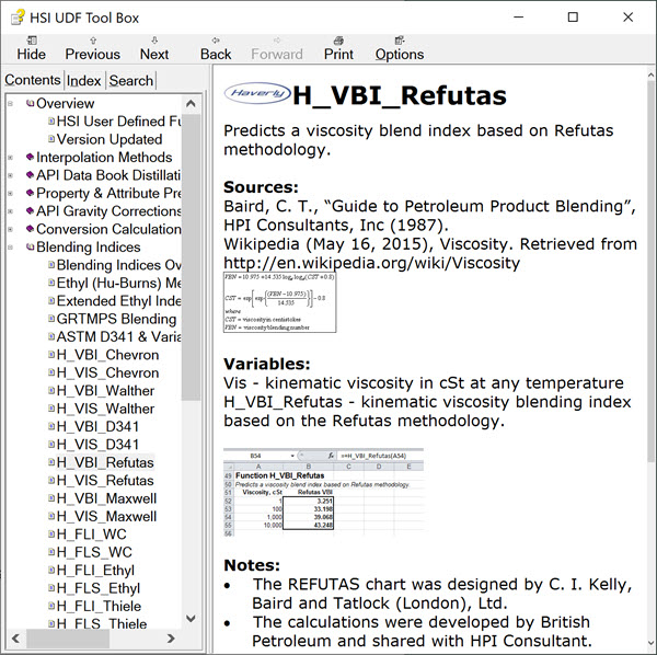
The companion function H_VIS_Refutas converts back to viscosity. If you have the add-in active you can use the functions to do the conversions without writing out the formula yourself. They are also built in to our PSI-2 tool, so you can use them efficiently in your unit simulators (and they will work even if the add-in is not active on the machine). Otherwise, an on-line search will reveal various possibilities.
How do you know if an index is any good? Indices are statistical constructs based on measured values of components and blends. Whether one works well for you will depend on how that underlying dataset – the range of values, the types of components, blend recipes – corresponds to what you have. For example, if an index for some property was developed decades ago, when products had higher sulphur contents it may not work as well for modern low sulphur fuels as one that was developed more recently. So you need to do some monitoring and testing to check any index that you choose – an exercise worth repeating when there are significant changes in your component pool.
When selecting an index to be used in an LP or SLP model, it is better to have one that blends on the same basis as the material balance so that the recursion doesn't need to deal with a density effect as well. Refutas blends by weight, which is why the example is done with tons. If your model balances streams in barrels or cubic metres, you will probably be better off with one that blends by volume. It will be most convenient if the same formula is applied to all components and if it works over a wide range.
In GRTMPS, users may indicate an index for a blended property by selecting an equation type and setting the co-efficients. Refutas viscosity, for example, can be done with equation type 2.
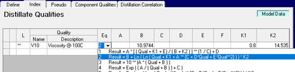
If you are using Table based input, the index is set in 500.8 or 600.8. Using “**” for the location code means that the same index applies to the property at all locations in the model, which is sensible if there is any transfer of blending components between sites.
There are currently 16 equation types. If you chose an index from the UDF set, the help file includes a note on which GRTMPS type can be used to implement it. If you have something else and can’t see which to use, please ask. It has been some years since we have come across an index that can’t fit into one of the existing ones, although you may need to do some clever reformulation to see it. (I appeal to Richard Tan when I get stuck, as he is quite good at working these out.) There is a certain art to realising which elements can be eliminated by setting a co-efficient to 0 or 1. Power functions, such as the widely used RVP index “psi ^ 1.25” can usually be done as a type 1. (I leave the setting of the A,B,C etc. values for that as an exercise for the reader.).
If you are using a nominated equation type in GRTMPS, then you enter your component data and specifications as measured quality values. The conversion to index is done as the data is processed and then back to quality after the solution has been found. That is, the input data and reports are in quality and the matrix and the recursion tracking are in index. (If you have an index that does not apply the same formula to all components, then you need to pre-calculate the values and carry the index as an additional property.). So the blending side is very simple.
The interaction between indexed qualities and process units – both feed and rundown streams can be more complicated. If you are using old-fashioned static delta-base unit operations and quality transfers, then you need to remember to formulate your base and shift vectors in terms of index. If you are using Adherent Recursion (either in-model or with a PSI workbook) then normally pool properties that are taken from the solution as inputs to the calculations are in index. Properties of output streams can be returned to the model in quality or index as set on the Adherent Recursion panel ($REALBASE in TABLE 200.0). The detail of this is something for a future note – or attend our advanced process unit modelling course and all will be explained!
Indices make it possible to handle many more properties than simple linear blending, but they are still not enough to do a good job in every instance. Octane, for example, does not appear to have any effective simple index method. Ethanol is an awkwardly behaved component with respect to many properties. Evaporation / distillation specifications are awkward. There are also properties that don’t blend well themselves, but can be predicted from others that do, like VLI and K-Factor. For these properties and others like them non-linear blending formulations on the blends are more useful – with delta-base-like approximations that are updated between recursion passes until the final values agree. Also a topic for later.
From Kathy's Holiday Villa, Plemmirio, Italy 2nd October 2019.
Comments and suggestions gratefully received via the usual e-mail addresses or here.
You may also use this form to ask to be added to the distribution list so that you are notified via e-mail when new articles are posted.