Does it make any difference, asks a reader, if you use a FIX or equal MIN/MAX constraints? Why fix anything in your model, because if you do, you’re not optimizing it? There are, of course, situations where you do want to force an option to a particular value. You might have already committed to sell a particular amount of a product and be looking for the most efficient way of producing it. You might be interested in the relationship between an operating parameter and feed pool quality and so running a series of cases at different values to generate a graph. You might be doing back-casting or trying to understand why two solutions are different. So what difference would it make if you did the target as a FIX or as equal MIN/MAX constraints? One very obvious point is that it takes two constraints to do both a MIN and a MAX, while a FIX only adds one row to your matrix – and small is always beautiful when it comes to speed. (In the case of purchases and sales in GRTMPS models, limits on single options are done as vector bounds, and so the difference in matrix structure is minimal.) But is either one or the other easier to solve, and does it affect the marginal values?
As a small experiment, I ran the volume demo model base case – which currently does not hit very many unit capacity limits -- and then set up a case constraining the units to run to the optimized daily rates (By the way, I used Report Generator II to write an SSI sheet so I didn’t have to type them in.) I set up one case with all FIX limits and another with MIN and MAX set to the same value. Both problems converged to a value similar to the original open case. The MIN/MAX case needed 8 passes to converge, the first 5 of which were infeasible. The FIX started with 3 infeasible passes and finished in 7.
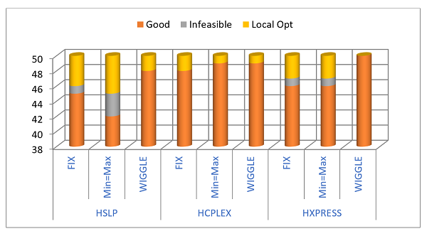
While this is a hint that the FIX method is more efficient, a single comparison is not much use in a system where there is natural variability; the differences in the matrix may simply have pushed the recursion down a different path (See Note #19 SLP and Chaos). We need more data. So, I ran 50 cases on each configuration, using the Multi-Start tool to generate alternative initial estimates for the recursed qualities and their error distributions. I based them on the final qualities (the 181 file) of the original unconstrained base case so that the same values were used for both sets of runs. Fix and Min=Max could then be compared on the number of cases that converged to a good solution, passes needed and the number of infeasible passes. The demo models are normally very stable in objective value, but the multi-start runs for these constrained cases included a very poor local optima, where an infeasibility purchase for premium gasoline is active. (An interesting example of how a “get out of jail” card can sometimes make things worse.) The number of times this turns up is also a useful metric. Once again there was an indication that the FIX method was better than the MIN=MAX.
| % Good Solution | Infeasible Cases | Local Opt Cases | Passes (mean) | Infe Passes (mean) | |
| FIX | 90% | 1 | 4 | 6.1 | 2.6 |
| MIN=MAX | 84% | 3 | 5 | 6.2 | 2.6 |
The demo models use our HSLP optimizer by default but most larger models are run with H/XPRESS or H/CPLEX. These both have sophisticated pre-solve algorithms that are supposed to tidy up the matrix before it is optimized. This might make a difference to the impact of the constraint structure, so I repeated the tests with each optimizer.
| % Good Solution | Infeasible Cases | Local Opt Cases | Passes (mean) | Infe Passes (mean) | ||
| HSLP | FIX | 90% | 1 | 4 | 6.1 | 2.6 |
| MIN=MAX | 84% | 3 | 5 | 6.2 | 2.6 | |
| H/CPLEX | FIX | 96% | 0 | 2 | 6.1 | 2.2 |
| MIN=MAX | 98% | 0 | 1 | 6.2 | 6.2 | |
| H/XPRESS | FIX | 92% | 1 | 3 | 5.8 | 2.1 |
| MIN=MAX | 92% | 1 | 3 | 5.8 | 2.1 |
Both of these more powerful optimizers do better than HSLP – with fewer infeasible cases and fewer local optima. With H/XPRESS, the pairs of FIX and Min=Max runs appear to be identical. This suggests that it recognizes when a pair of MIN and MAX constraints are effectively a FIX. H/Cplex however, found the local optima for different cases in the two designs, and so clearly does not do that, but the difference between designs is otherwise minor.
Wiggle Room
There is, however, a further additional option available if you set up two constraints. They don’t both have to be exactly equal to the target. You can give the model a little “wiggle room” – and this is probably particularly useful when you are constraining a number of items as it is all to easy to forget about degrees of freedom and numerical accuracy and end up tying the case up in a knot. So I added another set of runs, setting the minimum to 99.5% of the target maximum. This is clearly very helpful in avoiding infeasible solutions, and it also reduced the number of local optima. There is still no difference in objective value for the good solutions as the deviation permitted is so small.
There is, however, a further additional option available if you set up two constraints. They don’t both have to be exactly equal to the target. You can give the model a little “wiggle room” – and this is probably particularly useful when you are constraining a number of items as it is all to easy to forget about degrees of freedom and numerical accuracy and end up tying the case up in a knot. So I added another set of runs, setting the minimum to 99.5% of the target maximum. This is clearly very helpful in avoiding infeasible solutions, and it also reduced the number of local optima. There is still no difference in objective value for the good solutions as the deviation permitted is so small.
Marginal Values
But what about Marginal Values? Does the method have an effect on the reported incentives on process unit capacity? A problem with looking at the MVs in this situation became immediately apparent when I tried to analyse them. I had constrained most of the unit feeds to match the previously unconstrained optimal value - that is where the MV is zero. So if that target is hit precisely, the MV would be zero – and it often was. So I studied just the FCC feed limit as that was at its maximum in the original base case with, all runs agreeing, an incentive of 55.825 (+/- 0.001). The objective values were virtually the same for all the constrained cases that didn’t find the poor local optima, varying by less than 0.01%, so I was expecting the MV on the FCC feed to be fairly stable, but perhaps to occasionally show a negative value from picking it up from the Minimum side of the limit. A negative value – indicating an incentive to go below the target -- did turn up occassionally (on fewer than 3% of cases). But what was most striking, was the great variability in values across the good cases, ignoring the few negatives, even though the objective values almost identical, the other process units were also all constrained to target values, and there were only three crudes to choose from and one basic set of products.
But what about Marginal Values? Does the method have an effect on the reported incentives on process unit capacity? A problem with looking at the MVs in this situation became immediately apparent when I tried to analyse them. I had constrained most of the unit feeds to match the previously unconstrained optimal value - that is where the MV is zero. So if that target is hit precisely, the MV would be zero – and it often was. So I studied just the FCC feed limit as that was at its maximum in the original base case with, all runs agreeing, an incentive of 55.825 (+/- 0.001). The objective values were virtually the same for all the constrained cases that didn’t find the poor local optima, varying by less than 0.01%, so I was expecting the MV on the FCC feed to be fairly stable, but perhaps to occasionally show a negative value from picking it up from the Minimum side of the limit. A negative value – indicating an incentive to go below the target -- did turn up occassionally (on fewer than 3% of cases). But what was most striking, was the great variability in values across the good cases, ignoring the few negatives, even though the objective values almost identical, the other process units were also all constrained to target values, and there were only three crudes to choose from and one basic set of products.
| Marginal Value on FCC feed (FCF) |
Min | Max | Mean | Std. Dev | |
| HSLP | FIX | 32.46 | 88.40 | 43.22 | 12.69 |
| MIN=MAX | 3.31 | 109.24 | 42.47 | 28.36 | |
| WIGGLE | 16.69 | 55.83 | 43.03 | 13.09 | |
| H/CPLEX | FIX | 1.70 | 42.01 | 35.84 | 10.49 |
| MIN=MAX | 5.02 | 157.17 | 66.29 | 27.20 | |
| WIGGLE | 16.70 | 56.35 | 51.04 | 11.39 | |
| H/XPRESS | FIX | 32.51 | 88.40 | 44.90 | 15.71 |
| MIN=MAX | 32.51 | 88.40 | 44.90 | 15.71 | |
| WIGGLE | 17.55 | 55.83 | 48.48 | 10.33 | |
As you can see the incentive went from as little as 1.70 to as much as 157.17 As there is quite a difference in the minimum and maximum values in the different cases, it is not surprising that there also a fairly wide range in the mean value. What I find most interesting, however, is the differences in standard deviation (Excel formula STDEV.P). This shows that some sets of values are more variable about their mean than others. The highest variability is seen on running HSLP or H/CPLEX with MIN=MAX constraints. This variation reduces when the problem has a little room to work in, but the most stable values come from using FIX constraints. H/XPRESS works differently, since the MIN=MAX produces exactly the same answers as the FIX method – both having an intermediate level of variability. Again, the WIGGLE cases contain the least variability. How much does the objective value actually change if the constraint is relaxed? I haven’t checked yet. Something to explore for a future note. It is possible that this behaviour is an artefact of the way I constructetd the cases, or peculiar to this simple model. I have not seen this kind of analysis before and would be very curious about your results should you try something similar with your own model.
An Answer
Going back, however, to the original question: Does it matter if you set targets using one FIX constraint or a pair of equal MIN and MAX limits? If you insist on a hard target, then for H/XPRESS it doesn’t matter (assuming you don’t turn the pre-solve off). For HSLP and H/CPLEX you are probably better off with the FIX, as it appears to be a little more stable. However, it is probably a better strategy to set your targets as a pair of constraints with a small gap between an upper and lower limit. This “wiggle room” appears to increase the chances that you will end up with an optimal, valuable solution and a more stable incentive value.
Thanks to Herb Klassen for the question.
From Kathy's Desk, 2nd November 2017.
Comments and suggestions gratefully received via the usual e-mail addresses or here.
You may also use this form to ask to be added to the distribution list so that you are notified via e-mail when new articles are posted.