If you are working with GRTMPS database models and entering your data via the interface panels the older GRTMPS data table system may be something of a mystery to you. However since the database information is exported into these tables before being processed it can be very helpful to be able to recognize the connections between panels and tables. Debugging tools such as data check, run time messages and file compare all refer to data in the internal tables, so knowing how the names work will make you more efficient. Here is a brief guide.
OMNI, our language that is used to translate input data into a matrix for optimization, reads two kinds of input: CLASS and TABLE.
| A CLASS is a list of codes and descriptions. For example, here is the CLASS OBJ which will exist in all GRTMPS models. | 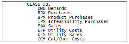 |
| Most of the data, however, is in tables. A TABLE is a named two dimensional array, with rows and columns very much like the data grids that you see in the user interface panels. Here is part of TABLE 200.0 from the Wt demo model. | 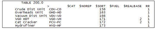 |
You can find out what CLASSes and TABLEs are generated for any data tab from the Help for that panel. Scroll down until you find the section “Tables Created”. This will show you an example and give some details. Here, for example, is the Help file for Process Unit Limits.
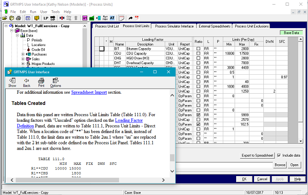
As you can see, the Process Limit information is primarily exported to TABLE 111.0. The column names in most of the tables will have some correspondence to those in the data entry grid, although they are not necessarily identical as they are here. The rows in the table are constructed by combining the elements that are filled in on the entry grid to create a unique data record. So here the entries in columns NAME, L and P on the panel give you the row names L+P+NAME [that is (LL)(PP)(LIM)].
To save you opening the Help file on every panel, here is a data tree annotated with the main tables generated for many commonly used data tabs at that node. You should note that there isn’t a specific one-to-one correspondence between panels or data grids and tables. Some panels write data to several tables; some tables are the result of inputs in multiple panels.
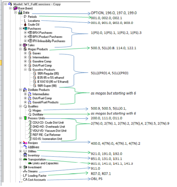
Some of the tables have fixed names, others are data driven and use the codes of model elements. These variable parts are indicated above in brackets: (PS) for Cost Accounts Used for P/S, (LL) for locations, (PRD) for streams of type prod, mogas or dist and (TN) for the 2-ltr part of process / unit recipe names.
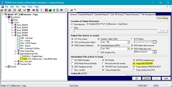
You can see the ones that are generated from your model data in the DB$ file, which will appear in the “Intermediate Data Files” sub-section of the output node, if you have marked it to be kept.
The first character of a numerical table name indicates the broad category of information to which it belongs:
| 1: Case Data | 5: Mogas Blending | 9: Definitions |
| 2: Process Units | 6: Distillate Blending | R: Report Configuration |
| 4: Recipe Blends | 8: Transportation, inventory |
The Case Data tables start with a “1” and are usually generated from panels where a period must be indicated, such as the Purchase or Sales Summary grids. Limits and prices are almost always exported to these tables. The higher number “Master” tables generally contain object definitions, such as the list of streams [911.0], and relatively constant aspects of the optimization problem, such as process unit yields [2(TN).2] and blend specifications [(5/6)(LL)(PRD)]. These tables often contain location, but not usually period, specific information.
Within each series there is a hierarchy of tables moving from general to more specific information. In most of the table series the “point zero” table has the job of defining options, while the other sub-tables link those options to other objects, such as group limits and loading factors.
| Here is the set of tables that can be generated for a Cost Account that is used for P/S. If, for example, you have a Revenue Cost Account, SAX, that is marked "Used for P/S" it will be a choice on the Sale Summary panel and the sales you enter for it will be exported to table 1SA.0 with their prices and limits. The other tables will only exist if you have made use of these more complex relationships - if there are group limits associated with those sales, or connections to loading factors, for example. | 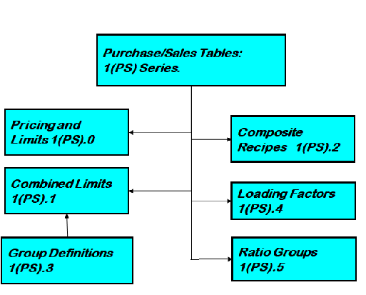 |
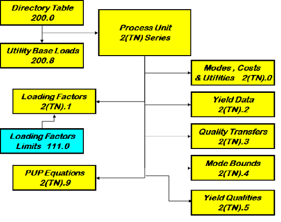 |
Here is the process unit series. The “Process Unit List” becomes the directory TABLE 200.0, as shown above. Each of the active units in your list has a node on the model data tree, where the data defining how it operates are entered. These are exported to the set of unit specific tables, 2(TN).x, where TN is the 2-ltr code appearing after the hyphen in the unit name. The Cat Reformer, REF-RE, will generate a set of 2RE TABLEs, each containing different sub-sets of the unit data. So the “Define Modes” creates the 2RE.0 Table. The Operations panel generates a table for each type of row that exists. Utilities and costs go into 2RE.0, Loading into 2RE.1, Yields into 2RE.2, Quality Transfers into 2RE.3. Bounds go into 2RE.4. The Yield Qualities panel makes 2RE.5, while the Adherent Recursion construction primarily goes into 2RE.9. The "point-zero" will always exist for any active unit, but not all units have data of every type so only some of the sub-tables will be written. |
| Their are two parallel sets of blending data for mogas and dist type products, pools and components. The tables come in three levels: model wide, location specific and product specific. This data is spread more widely through the database than the process unit information. Some is exported from the Streams panel [(5/6)00.0], some in qualities [(5/6)00.9, (5/6)00.5, (5/6)(LL)0.1 etc.] and some on the individual blend nodes [(5/6/)(LL)(PRD).4)]. As with the P/S series and the process unit tables, some blend tables are more common than others and some are very seldom used and won't appear in your data. | 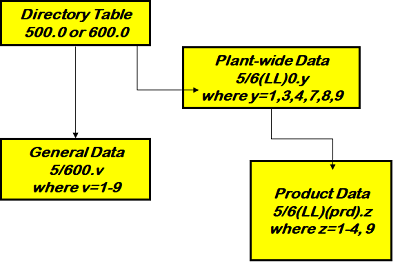 |
The table structures for recipes, inventory, transportation and investment are rather simpler and you should find it reasonably straight-forward, so I won't take the space to lay them out here. For a complete description of the CLASSes and TABLEs used in GRTMPS have a look at the Modelling Reference Guide (accessible under the Help Menu).
Now lets put our grasp of the table name system to some use.
Suppose you have the run time error “*E* Quality N2A in TABLE 2RE.1 Limit RN3 not recursed for RD#. Run aborted.” The table name starts with 2 so you know this is related to a process unit named 3-letters-RE. So your investigation should include the operations panel for that unit (and also of course the quality data for RD# and the Loading Factor definition for RN3.)
If you run a datcheck report and see
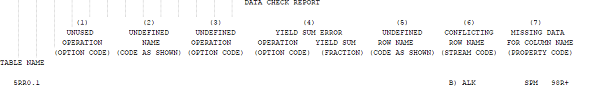
the "5" tells you its a mogas problem. It's a location, but not product specfic table, so navigate to the Mogas Qualities node and have a look at the component data for location "RR".
You should also now be able to gather some useful information about the differences between cases by using GRTMPS File Compare (Tools menu, or right-click in the Output tree) to see what is different in their DB$ file. File compare is a big enough topic for an article in its own right, so watch this space.
From Kathy's Desk 11th Juy 2017.
Comments and suggestions gratefully received via the usual e-mail addresses or here.
You may also use this form to ask to be added to the distribution list so that you are notified via e-mail when new articles are posted.