 |
Where does negative sulphur come from? If you are fortunate enough to only ever see converged solutions to very well-behaved models, then you might not have ever seen negative sulphur, or percent distilled values above 100, or benzene content below zero – but these impossible properties can turn up in distributed-recursion models, even in optimal solutions. |
Consider a stream that can be put into inventory or transported to another processing site, without anything else being added to it. Whatever the sulphur content of that stream, it should have the same value in the next period and at the other location. But if the source a blended pool or a process unit yield with variable properties, and the split between transport and inventory is not pre-determined, there is no linear equation that can impose that “same” condition. However, since this is the classic pooling problem, it can be optimized via a series of linear approximations. (See How Distributed Recursion Solves the Pooling Problem.)
This is, however, an imperfect system, as the qualities are not automatically correct. They will only be right when a solution is found that maintains consistency between assumed and actual values. (See Does Convergence Matter?) The approximations built into the model can give rise to negative sulphur or other impossible properties on recursion passes where unconverged solutions are produced. Let’s add some numbers to our simple example configuration. The sulphur value of the source and the pool dispositions are not known in advance, so we need some initial estimates. These are used to set up the equations for tracking its value in the destinations and satisfying any specifications in the first linear matrix.
Assume that the source stream has 10 ppm sulphur and is equally likely to go to inventory or be transported, a 50/50 split. Imagine that in the optimal solution to this approximation, the stream came out with 12 ppm sulphur. Although we know that the destination pools should also have come out as 12 ppm, their sulphur values will depend on the accuracy of the assumed error distributions. Because of the Distributed-Recursion structure in the matrix, the sulphur of each destination pool is determined by the assumed fraction of the error divided by the actual tonnes received. (In the matrix, the error is multiplied by the amount of pool produced, but if we consider just 1 “unit” of material, whatever that is, then the distribution factor is a stand-in for the quantity.) The average actual value of the pool in the next period or at the other site in this solution is:
= Assumed Quality + (Quality Error * Assumed Distribution)/Actual Distribution.
If the pool was actually divided evenly between the two uses, then each of the destination pools would have perceived the sulphur as 10 ppm + (2 * 0.5)/0.5 = 12 ppm. That would be a converged solution because the pool sulphurs all match. However, if the pool did not distribute evenly, as assumed, but split 40/60, then the destination pools would not have matched the source (or each other):
10 + (2 * 0.5)/0.4 = 12.5 ppm and 10 + (2 * 0.5)/0.6 = 11.6667 ppm.
One pool has too much sulphur because the error is divided over a smaller amount than assumed, while the other has too little because it did not receive enough error. This is not a converged solution, and another approximation needs to be tried. Notice, however, that the sulphur balance is maintained:
0.4 * 12.5 + 0.6 * 11.6667 = 12 ppm overall.
So far, the values are reasonable, but when optimal sulphur is less than assumed the error is negative. If the actual distribution moves far enough from the assumed, a negative overall value can be produced for one of the destination pools. Suppose on the next pass the sulphur drops from the assumed 12 to 8 ppm, and the tons are split 90/10.
- The destination sulphur values would be
12 + (-4 * 0.4)/0.9 = 9.78 ppm and 12 + (-4 * 0.6)/0.1 = -8 ppm.
- The overall sulphur balance is still maintained: 9.78 * .9 + 0.1 * -8 = 8.
- The overall sulphur balance is still maintained: 9.78 * .9 + 0.1 * -8 = 8.
Bad qualities can also be generated in delta-base process units. If, for instance, there is a delta vector that says sulphur goes down as severity goes up, it could run further than intended taking the output property below zero. The negative value often makes the stream a very desirable material. It could be used to blend away a much higher sulphur contribution from other components going with it into finished products or unit feeds. This can create a strong incentive to generate such values, particularly if there is no economic impact of the excess sulphur on the other the destination - say if it is just being sold or left in inventory.
The algorithms that are used between recursion passes to update the approximations can apply a dose of reality to weird solutions. Without the requirement of expressing rules as linear equations, we can, for example, take into account that these destination pools must always match the source. If you are using a linked process simulator to update your deltas on each recursion pass, that should also reset the model to a more realistic position. (Unless your simulator itself predicts negative sulphur, in which case some improved filters and maybe a skip test, or even a bit of “back to the drawing board” is in order.)
However, these impossible quality values can still hamper the optimization. If they keep reappearing in the solutions despite more sensible assumptions being used, the model is unlikely to converge. An effective countermeasure is adding a specification: Sulphur >=0, to the pool where the bad value is turning up. It may seem like you are stating the obvious, but the optimizer only only knows what it finds in the matrix equations – it doesn’t understand physical reality – its all just numbers. A specification like this is a way of indicating the limitations of the approximation's match to the original problem. It establishes a “trust region” where solutions are possibly useful, and makes infeasible those that cannot be.
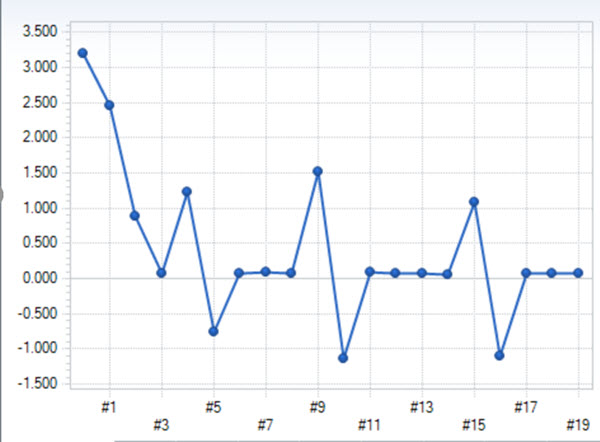
Use the Recursion Monitor to identify pools that are prone to bad values and put in just a few of these trust specs to start with. Controlling one property on a pool will often prevent other bad values as well, since the new specification limits the shift in distributions or blended property on each pass. But you probably don’t want to put them in everywhere by default. We don't want to make our models bigger and slower than necessary. You may also find with too many constraints, that it might not be able to get started - finding that first optimal pass. Sometimes a little bad behaviour is needed to get the optimization process out of a hole.
You wouldn’t expect to see this sort of specification constraining in a converged solution, but that doesn’t mean it isn’t doing something important. Use the Recursion Monitor again to see if it is having an influence on previous passes – in which case it is helping you fight the forces of chaos (See SLP and Chaos) and you should leave it be!.
Comments and suggestions may be sent via the usual e-mail addresses or here.
You may also use this form to ask to be added to the distribution list so that you are notified via e-mail when new articles are posted.
From Kathy's Desk, 4th February 2019.