Swing cuts are a well-established method for representing flexibility in cut-points on refinery distillation towers. While direct cut-point optimization by dynamic re-cutting will give you a more accurate quality prediction, not everyone has access to both GRTMPS and HCAMS, so it is still useful to know how to configure swing cut units. The complication in setting this up is that the cut-point is determined by how much of the swing has blended up or down into the adjacent core cuts, rather than directly on the unit where we want to control and report the optimal values.
In case you are not familiar with swing cut modelling, lets start with a look at what that is.
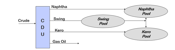
Each crude going into the unit is represented with a pre-cut yield pattern. “Naphtha” and “Kero” are the core cuts. They represent the boiling range that always comes out of that side draw. The “Swing Pool” is the material that could be distilled into either naphtha or kero, depending on the temperature achieved at that point in the tower. It does not represent an actual physical stream on the plant. Swing cut modelling is usually done with the assumption that all the feeds are being run at the same time in the same operating conditions. So the contributions from every crude are collected together into a single pool of each cut. The swing cut pool is then allowed to blend up to the naptha pool or down to the kero pool. The portion of the swing that blends into each core cut determines the effective cut point. If the swing pool blends up, the naphtha end boiling point (EBP) becomes a higher temperature, if it swings down the Kero initial boiling point (IBP) becomes a lower temperature.
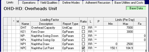
To control the cut points as an operating parameter and report them with the unit, there needs to be a connection between the blending and the process unit operations. There is an example of how to do this in the overheads unit (OHD) in the WT demo model unit. There are, as usual, other constructions that work, but I like this one because it puts all the controls and cut point information in the process unit for easy maintenance. The illustrations are all taken from the database input model, but the table based demo model has the same structure if you want to see it in that format.
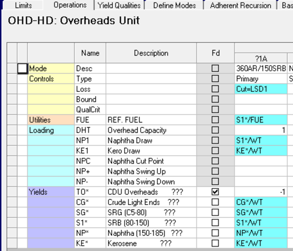
This is the generic base mode for the unit that will be filled in for each crude:
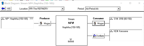
The Naphtha 150-185 degree (Centigrade) yield stream is a swing. If you select it in the block diagram you can see that the crude specific NP* is collected into the pool NP#, that blends into the pooled SRB and Kero cuts on either side.
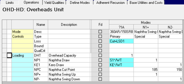
To track the cut point between SRB and Kero, you need some loading factors that count the amount of swing pool that is blended into each. Below shows counting into NP+ for the NP# pool blended up into S1# on its Gasoline Product node [TABLE 511S1#.3]. Using a "+" in the name helps me remember which way the swing is going. Note I am using a negative entry here. There is also an entry on KE# in the distillate section [TABLE 611KE#.3] for factor NP-, as this swing crosses the divide between gasoline and distillate components.
On the process unit these factors are used to drive operations N1+ and N2- to be equal to the amount of the swing in each direction. These modes need to be type Special so that the cut point average is calculated and reported correctly. [If using table based input, a non-alphanumeric 3rd character in the mode name, such as the “+” and “-“ used here mark a special mode – or $QTYPE can be set to 2. See the GRTMPS Modeling Reference Guidel for details.] They have a positive entry on the loading factors that are counted in the blending.
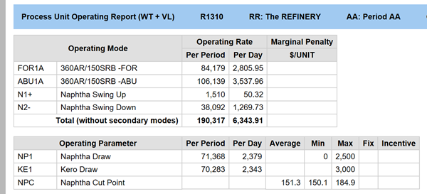
The average end point for the Naphtha will be calculated on Loading factor NPC, which is defined as an Operating Parameter [TABLE R07.1]. The swing cut goes from 150 to 185. So when the swing pool has blended up making the SRB longer, the cut point moves towards 185. While the down swing makes it shorter, moving it towards 150. If the swing split in half, the cut point would be 167.5. To count and control the total amount of SRB there is loading factor NP1 which takes the core cut yield on the base mode plus the amount blended up on N1+. For total Kero, KE1, the N2- activity is added to the base yield.
To make this work the NP- and NP+ loading factors musts be fixed to zero, as below. The cut point can now be constrained to any value between 150 and 185 (anything outside that range would mean that the model could only be feasible if the unit wasn't running.)
To help with convergence it is good practice to set the cut point constraint to just inside the value possible so that at least a little bit of the swing must go each way. This keeps the connection between the swing qualities and the core pool active so the recursion is less like to simply alternate the destination of the swing from pass to pass, something which often happens. If you are having problems with convergence check the distribution of the swing pool in the recursion monitor. You may need to constrain the stream disposals or qualitiesl more or use step bounding to get it to settle down if it is bouncing back and forth.
With this configuration the cut point operating paramters can be reported on the unit pages. This is the operations activities so you can see how the average cut point has been derived.
With more draws and swings, you just have to multiply up the structure. Some core cuts will have swings contributing to both their top and the bottom, but just set up each one in the standard manner and it will work. Things do get more complicated when a pool containing a swing is fed to another separation unit. For example, the atres pool from an atmospheric tower will be fed to the vacuum tower. Normally, this is modelled by de-pooling the residue back into its crude specific parts so that they go through the correct vectors with yields etc. generated from assay data using the atres IBP as the start of the column. If that feed pool also contains swing material, then the vacuum unit will need to have vectors to handle that material as well, but you don’t know its IBP in advance. So you will have to make some assumptions, and perhaps add some delta vectors to adjust the qualities based on the optimized cut-point …. or you could just do dynamic cut point optimization with HCAMS direct!
Thanks to Jean-François Sirinelli at Axens for the question which inspired the note.
Comments and suggestions may be sent via the usual e-mail addresses or here.
You may also use this form to ask to be added to the distribution list so that you are notified via e-mail when new articles are posted.
From Kathy's Desk, 17th January 2019.