19) Successive Linear Programming and Chaos

A butterfly flaps its wings in the Andes and your model optimizes to a completely different crude slate.  What? Were you expecting a comment about the weather?.  This kind of instability is a characteristic of “chaotic” systems.  Not in the sense of disorganized, but in the mathematical use of being very sensitive to initial inputs with no clear or systematic connection to changes in outcomes.  Weather is probably the most commonly cited example of a chaotic system.  Turbulence in air or water is another.  Since Successive Linear Programming models are sometimes unstable and find significantly different solutions in response to minor changes, they can also be described as chaotic in this sense.  Unlike weather or turbulence, however, it is just the optimization technique which is chaotic not the refinery processes etc. that are being modelled (at least I hope so).

SLP optimization shows its chaotic side when you change the order of streams or qualities and solve to an alternative solution, even though the mathematics of the problem are the same.   When you take out a crude that wasn’t active, and the answer changes.   Or if you add a minimum sale to a model and it sells just that much, even though it previously sold more.   It is particularly irritating when the model loses money as a result of a change that you did not expect to have such an effect.  Surely it should have been able to find the better solution we already know about! Why does SLP do this to us?

 

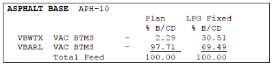
Although the demo models are reasonably stable, we can still use them to learn something about how this chaos happens.  Consider the volume demo model as installed.  The sale of LPG is at the minimum 200 BBL/day for all three locations.  So you might think you could just change the limit from MIN to FIX without affecting the result; after all this solution would still be feasible.

But you will end up with a different answer.  For example, the composition of the Asphalt Base product changes from being predominantly the vacuum residue of Arab Light, to a 70/30 mix of Arab Light and West Texas.  There is a corresponding shift in the feed to the Visbreaker that maintains the material balance.

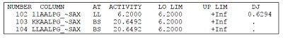
We don’t normally look at the early results in any detail, but the key to the impact of this change can be seen in the solution print for the first pass, which is in the LST file.   In the original case, in this first solution, only the LPG sales at 11 are at LL, the lower limit.  More is sold at both KK and LL.

 

 This solution would not be feasible when the limit is changed to a fix so the optimizer will have to do something different.  The SUM files show that the two runs do indeed have a different objective value on the first pass.

BASE CASE Step: Model Generation        End OK       :00       :07 Step: Simulator Generation        End OK       :00       :07 Step: Recursion Pass 00        End OK       :00       :07 Step: Optimize  Pass 00        End OK       :01       :08  OPTM   1746.7432      Step: Simulator Pass 01        End OK       :00       :08

FIXED LPG CASE Step: Model Generation        End OK       :01        :07 Step: Simulator Generation        End OK       :00       :07 Step: Recursion Pass 00        End OK       :00       :07 Step: Optimize  Pass 00        End OK       :01       :08  OPTM   1785.1341      Step: Simulator Pass 01        End OK       :00       :08

And there we are, starting off the search for a solution by heading in a different direction.  Remember that SLP works by solving a series of linear approximations (the “iterates”) until it converges on a feasible solution to the non-linear problems.   The first LP is created using your initial estimates, but in the subsequent ones these assumptions are updated based on the solution to the previous.   A different solution on any pass means a different LP on the next, means a different solution, means a different LP and so on.    If the economic drivers are strong and the options distinctive, the recursion process may ultimately arrive back at the same point, or at least one of similar value.  The demo models don’t include a lot of optionality so they do usually converge to the same objective.   Real models with more possibilities often don’t.  That’s not necessarily bad news, of course, because sometimes they find a better answer than before.

 

But why would something as simple as changing the order of the streams or qualities change the recursion path?   You are optimizing exactly the same LP problem at the start, so you shouldn't you find the same answer?  LP problems do have only one optimal solution – that has always been part of their appeal.   How can it go in a different direction?  It can because the  “only” applies to the value of the answer, but not the details of how that money is to be made.   Refinery optimization problems are often rather “flat” – meaning that there are many similar alternatives that produce the same amount of money.   You might, for example, be able to swop the components around between various grades of gasoline and still produce the same amount of product.  Or you could buy a mix of crudes that gives you the same quality as some particular single grade.    Which solution the optimizer finds depends on the choices that it makes about which variables to set (the “pivots”) as it progresses towards an optimal solution.  Simple descriptions of the Simplex algorithm will say that it chooses the one that adds the most value to the objective function.  However, the optimizers applied to large models use “partial-pricing” strategies for speed. The price calculations are done only for a sub-set of the variables each time a pivot is chosen.  If you change the order of the equations, add or remove structure (even if it can’t be active in the solution), you can change which variables are tried and therefore end up with a different one of the alternative solutions.  Using a basis file also changes the pivot selection.  

 

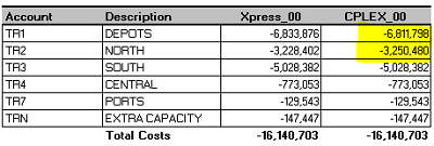
Different optimizers have different algorithms for choosing which variables to include, so this is an easy way to illustrate this point, even with the demo models.   I ran the Distribution demo model with H/XPRESS and H/CPLEX.  They agree that the optimal value for one pass is 16140.703,

 

but there are differences in the cost breakdown,	that reflect different choices in the routing of supply.

 

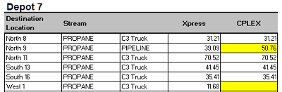For example, in the solution from CPLEX more Propane is sent from Depot 7 to North 9 and none goes to West 1. The second iterates would have assumed distribution factors based on these previous destinations. Those second matrices would, therefore, not be the same so the SLP optimizations would be following different paths. 

 

 

What can you do to avoid butterfly effects?  Some suggestions:

 

Be aware of the possibility of alternative solutions and learn to live with it.  Accept and understand that there are probably multiple reasonable strategies, often with similar economic outcomes.  Don’t put too much value on the details of any one solution.  If you do a number of runs for the same problem with Multi-Start, you may find some of these other options and you can use them to understand viable alternatives to your base plan.  Does it always  buy a certain crude, or does the grade show up only occastionally?   You can also deliberately look for these alternative plans by blocking out active options, such as a particular crude or transport routing and optimizing again for the next best choice. 

 

And don’t forget, you can sometimes harness that butterfly and use the chaos to your advantage.  Having trouble getting an optimal / converged solution?  Model ignoring some useful looking options?   Make a minor change and see what happens – you might just be able to nudge it out of a rainy day and into sunnier weather.