If you added a minimum to the objective function, would it make the model solve to the better answer? The idea is very appealing and there was a fad in the late 90’s for adding a replica of the objective function row, constrained to a something nearer the better value. This feature is still available in GRTMPS. It can be activated on the Advanced settings on the Case Node.
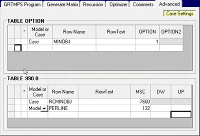 |
The MINOBJ option activates the feature, while the target value goes in RCMINOBJ. As GRTMPS sets up the LPs as minimization problems, profitable solutions have negative objective values. I have entered -7600 as that is closer to the -7615 solution than the -7325 from the less constrained case. If you are using table-based input, MINOBJ goes in OPTION and RCMINOBJ goes in 990.0. Both elements of this became available via the user front end with the release of v5.8. If you are running an older version that does not have the new TABLE 990.0 grid, the RCMINOBJ value has to be entered via Table-based input in an additional data file. |
| With MINOBJ active, an XXDOLLIM row is added to the matrix, as can be seen in this extract from the "ROW" file. Each contribution to the XXXDOLLAR objective row is repeated in this limit. GRTMPS uses a system of Cost Accounts for expenses and revenues of different types, so the rows are actually rather simple. Each column represents a sub-total on the account. (The prices are in the rows that drive the sub-totals). As a consequence of writing the matrix as a minimization problem, our minimum target value needs to written as a MAX limit. |
Matrix GRTMPS has 3631 rows and 3231 columns Row = XXDOLLAR Type = OBJ Row = XXDOLLIM Type = MAX RHS = -7600.00 |
So, now the model has been told – Begone annoying local optima, find me a better answer or else!
Our intention was to drive the model to an optimal converged solution of at least $7600, but what you get is:
**** T H I S S O L U T I O N W A S I N F E A S I B L E ****RECURSION SUMMARY
| PASS | ITERATIONS | SOLLUTION STATUS |
OBJECTIVE FUNCTION |
| 0 | 1709 | INFE | 760000 |
| 1 | 516 | INFE | 760000 |
| 2 | 113 | INFE | 760000 |
| 3 | 147 | INFE | 760000 |
| 4 | 254 | INFE | 760000 |
| 5 | 203 | INFE | 760000 |
Adding this constraint to a matrix that was solving to a worse value just makes it infeasible. This should NOT be surprising. The whole point of defining planning problems as Linear Programmes is that LPs have only one optimal solution. The Simplex algorithm steps through the variables and constraints in the minimization problem to find the smallest objective value. There may be more than one combination of column activities that produce this value, but the value is the value. If that value isn’t as good as the target, the added row simply makes the problem infeasible. The situation doesn’t improve with the recursion passes. An SLP algorithm uses properties and distributions from each solution to generate the next LP approximation. Its purpose is to steer the process towards a solution that is not only converged but also profitable, but it can’t make much use of the target value in that decision process, because it can’t know the economic consequences of its assumptions until the LP is solved. That is, the target is somewhere where it does no good, and where it would help, we don’t have enough information to make use of it. So, a constraint on the objective value isn’t going to solve all your local optima issues (unless you prefer infeasible solutions to ones with bad values).
But people will tell you that that they have seen it have a good impact on a problem case and so regard it as something useful to do. If the fundamental thought behind it is not sound, how is it that it sometimes works? I can think of a few reasons:
1) SLP models are chaotic – Simply changing anything in the matrix can make it follow a different recursion path. Adding the extra row for the objective limit sends the processing in a different direction, but is no different from the impact you sometimes see when changing the order of the streams. It’s just different. Something that makes the model infeasible on an early pass is even more likely to have an effect on the recursion path because optimizers stop as soon as they detect that the problem can’t be solved. Starting from a bad position makes it less likely that a good answer will be found, but sometimes the resulting alternative path leads to a better destination.
2) Infeasible Passes are Processed Differently. The SLP algorithm’s rules for setting the assumptions for the next pass might use the optimization status as part of the decision process. While the simple principle is that you just use the previous values, an Infeasible status indicates that there is a problem with that information, so it is quite sensible to take that into account in some way. Even if the optimizer has worked out that it is only objective value constraint that is infeasible, the SLP still might make different decisions about the next pass values. For example, in GRTMPS, the Step Bounding system won’t activate until there has been at least one optimal recursion pass. This change in strategy will alter the path of the recursion process, such that you might end up with a different result.
3) The LP is Not Convex –The simplex algorithm requires a Convex problem. When translating data to a matrix for refinery planning problems, etc. we assume that we will end up with a convex problem – and do so pretty much all of the time since we are writing a linear approximation. But it is possible that some combinations of assumed values, constraints and numerical precision could generate a non-convex problem, where there is a gap or a dip in the edges of the solution space. Given such an issue, simplex can stop at a non-optimal solution as it can’t follow the boundary by linear extrapolation. In this case, an additional constraint on objective value could be having a real effect because it removes the non-convex bit of the problem from the feasible region. I think that I have seen such a matrix just once in my career (around 1992). It solved to a different objective value depending on having a starting basis or not – but as it as was a linear problem, simplex should have always found same answer, just with different numbers of iterations. I’ve always suspected this was a trade-off between product density and sales quantities for something that was be sold by both weight and volume, but never managed to prove it. I do note that it came from a refinery where the modeller believed in the power of the minimum objective, so perhaps they regularly had such issues owing to the nature of their sales contracts.
Nonetheless, even if it sometimes looks like a minimum objective value is resolving problems with local optima solutions from an SLP model, the effect is probably unspecific and could be achieved by any number of other changes. This is obvious (at least in retrospect after you have done the tests, as I did a few decades back) if you think through how SLP works. I’m not sure why anyone would bother with it for this purpose. Multi-start is a more convenient way of finding alternative solutions to a problem, now that we have so much computer power at our disposal. Doing a few dozen runs and keeping only the one with the best solution is an effective approach.
But if you want to set up an alternative objective function to minimize something else, such as carbon emissions, but make sure that a level of profitability is preserved, then a minimum on the net income will be a useful feature - and this is why there is some renewed interest in the option and we are making it easier to access.
From Kathy's Desk, 14th September 2023.
Comments and suggestions gratefully received via the usual e-mail addresses or here.
You may also use this form to ask to be added to the distribution list so that you are notified via e-mail when new articles are posted.