7) Initial Estimates: Effective Use of a 181 File

Distributed Recursion SLP models require initial estimates for the pool properties that are being optimized and the pool’s distribution factors*.  By default the pool property values are taken from the blending data and the error distribution is an even division over all the ways the pool can be used.  However, you can override these numbers by using a “181 file” as an additional input to the model.  

 

A 181 file is an optional output that can be marked for saving on the Output: General panel, as shown here, or on the Case: Recursion: Initial Values panel, as shown below.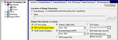

Ticking the box will result in a runid.181 file being written into the output folder at the end of the run.  You can also create 181 files using the Multi-Start tool; these will be in the MultiStart sub-directory of the output folder.

Choosing a 181 file
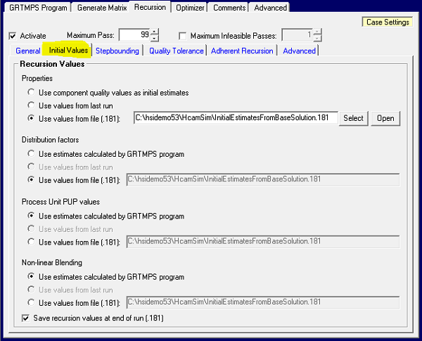
You use a 181 file by selecting it on the Case: Recursion: Initial Values.   You can also put 181 files in the Data File List.  A 181 selected via the Recursion panel is always read after the data files, so it will always have the last word.  If the file has been generated from a run with the same or similar data, this can help the solution converge sooner and sometimes find you a better value – particularly if the default values started the optimization off with infeasible passes or for multi-period models as the defaults quality estimates are not period specific.   If you are relying on a 181 file, it is a good idea to move it out of the output folders into another location so as to not unintentionally overwrite it.  In the example below I have copied the Base_00.181 file from the output folder into the data directory and renamed it to "InitialEsimatesFromBaseSolution.181" so I know exactly what it is. 

 

The 181 does not need to come from a run that matches the current model exactly.  It might, for example, include products that are not currently made, or not include a new unit.  It might have fewer - or more -  periods or locations.  When you are studying variations on a scenario, it can be a useful tactic, to use the 181 from your base case as a starting point for the alternate cases.   If you have a large complex model, you might be able to build up to a good set of starting values by running sub-sets of the model and using those 181s to jump-start the full run. For example, if you have a multi-period model, get a solution to the first  period and use that 181 for the full case.  If you have a refining plus distribution network set up, run the processing site alone and use that 181 for the whole model.   You can use multiple 181 files, selecting them via the Data panel, say from each refinery location in a corporate model, run as a stand-alone case.

Since initial estimates influence the path of the recursion, you should not be surprised if adding a 181 file changes the solution that is found. (That is one of the reasons we do it!).   In theory if you re-run a case from its own 181 file without changing anything else, then the first matrix (runid.MTX) should be the same as the last one in the original run (baserun.BCD), and it should only need one pass.  In practice, however, this only happens with simple models.  If the convergence criteria or tolerances in the model change over passes (see Case: Recursion: General or TABLE 990.0), then the same solution might not test as converged immediately.    The matrix will also not be the same if step bounding was active on the originating run.  Be aware, that if you are using a 181 from a very different case, it might make a new optimization worse.  This is more likely to occur if the differences relate to quality, such as the specification season – that is don’t run a summer case with a winter 181 or vice-versa.   181 files from infeasible runs are clearly not a good idea. And if you normally run your model with a 181 file and encounter a problem case, you should try turning it off or replacing it.  

Using Just Part of the 181
In the example above, I have chosen to use the 181 information for the pool property and distribution data, but not for the Process Unit Pup values or Non-Linear Blending.  I like to let the program recalculate those values based on the pool estimates so that they are definitely consistent with the rest of the model even if there have been some changes in the case data or the simulators.  If run time is a particular concern, however, you could select these too as then it is not necessary to run the simulators in the generation step.  

 

If you are running a “Basic” model with all the data in tables, then you tell the system to ignore the non-linear data in the 181 file by setting NOPUPADV and/or NOBARADV in TABLE OPTION.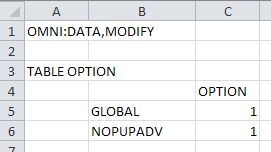

 

It is also possible to use the 181 file for property estimates but not for error distributions, by selecting “Use Estimates Calculated by GRTMPS Program” in the Distribution Factors section.  For basic models, use GLOBAL in TABLE OPTION.   The thinking behind using the default distribution system, where the pool is treated as equally likely to go to any destination, is to avoid biasing the solution towards or away from certain uses.  For example, if the 181 comes for a solution where a pool was not used in particular product, it would have an initial distribution estimate of 0 and so no connection between the actual pool qualities and the blend specifications.  Without that information flow, the pool quality might not be adjusted to be suitable for that product, even if that would be a profitable thing to do in the new scenario.

Consistency
If you want consistent results you need to use the same values every time.  If you use a 181 file, treat it like a part of your case data and make sure you put it in some location where it is not going to be overwritten.  I seldom use the “Use the Values from Last Run” option, as it will use a different file every time you run the case.  I only do this is when I am working on one that starts with a lot of infeasible passes and / or doesn’t converge.  I might run through a few cycles using the last run option until I have a good result.  Of course, if one of the runs is infeasible, I want to back up to the previous, so I change the run name each time.  If I find an effective starting point, I save that 181 file and select it explicitly.  
 
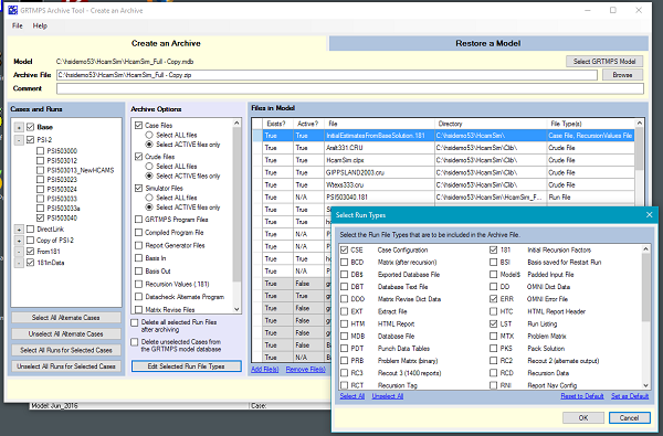
181 files that are listed in either the Recursion Initial Values panel or the Data Files list will be included when the model is archived, provided the case in which they are active is selected in the Cases and Runs section on the left.  The "Recursion Values (.181)" item adds a file to the list of what is to be archived but the choice of name is unpredictable and the file may not exist.  I suspect that this is a vestige of the way the "Previous Run" options were handled in GRTMPS 3.   If you want to keep the output 181s from your runs - perhaps to use them later - then you need to click on "Edit Selected Run File Types" on the bottom of the Archive Options section, and tick "181 Initial Recursion Values".    The files will only be included for the Runs that are selected.   In the example below, two 181 files will be included in the archive:  InitialEstimatesFromBaseSolution.181 because it is used as an input in case "From181" and  PSI503040.181 as the output 181 for a selected run.