I have extended one of the demo models to differentiate the sales of gasolines to different customers. The sales are represented as occurring at different locations, so that they can have distinct prices and limits.
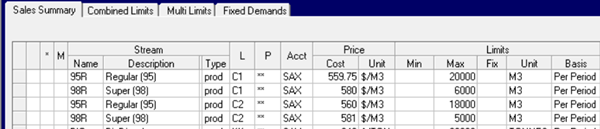
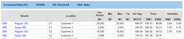
The model has no trouble meeting the demands for Regular (95) gasoline. There is not, however, enough Super (98) to satisfy both customers. (I made sure of that by putting a limit on the blending.)
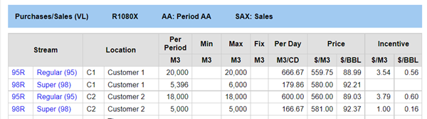
Naturally, the optimization favours Customer 2 who is paying more. What is left goes to Customer 1. (The incentive on the sale at C2 sale is, therefore, of course, the difference in price). Is this the best plan? That depends on the consequences of delivering less than promised. If there are penalties in place for failing to fulfil certain contracts, you should add these to the model so it can take those costs into account when deciding how to do the allocation, particularly if they differ for product grades or customers.
How easy it is to model a penalty depends on the conditions. “If you don’t supply x, you will need to pay y” sounds like an integer problem and may well require MIP techniques, but some rules can be formulated linearly. It is simple to model a flat-rate penalty that is a function of the amount that is missing. If Costumer 1 not only negotiated a better deal on price than Customer 2, but also included a penalty clause that compensates them with the difference between the contracted price and the spot market price for any shortfall, that should be taken into account. Let's say that currently works out at $2/m3 for Super (98). To represent the impact of that within the model, we need a variable that will be equal to the difference between the target (6000) and quantity sold (5396). If we set up an equation SOLD + SHORTFALL = TARGET then SHORTFALL would be equal to 604, which can then be multiplied by the cost.
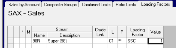
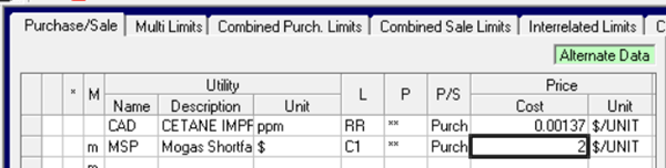
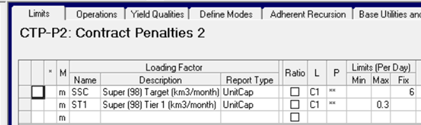
Such constraints are easily created in GRTMPS using Unit Capacity controls associated with dummy process units. The connection between the sale and limit is made on the Account node, on the Loading Factor tab (TABLE 1xx.4.)
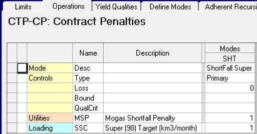
A process unit mode is used for the SHORTFALL variable.
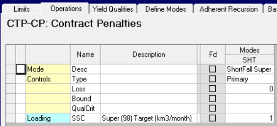
This is a primary operation and it has a loss of 0 --- both of which are triggers for various report tools for including units that have no material balance.
The capacity control has to be set to the target amount. We have a small issue here, since the sales limits are expressed as monthly totals in this model, while the process limits are per day. I could scale the amount by days, but I’ve chosen to set it as an “Unscaled” limit instead.
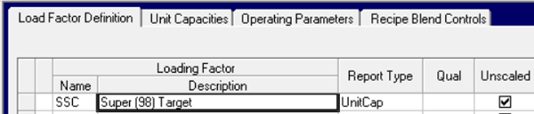
This means that the limits are not multiplied by days – nor is the normal RHS scaling applied so I have to do that myself, to make it consistent with the sale bounds as they end up in the matrix.
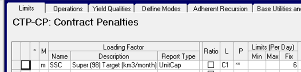
As there is only one sale involved here, this target limit makes the upper bound on the sale redundant, but that wouldn’t be the case if the target covers multiple activities.
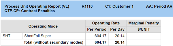
I check my structure by running the model again. Since the penalty cost hasn’t been added yet, the shortfall should still be there – and it is, as can be seen on the operations report.
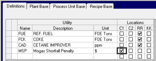
Now to add the penalty. Although this is a weight balanced model, since the gasoline is sold in volume, the count into the control is per m3, so the process operation is in volume too - no need to do any density scaling. While I could put the $2/m3 on a cost account on the unit operation that wouldn’t be very flexible. It's more convenient to model the penalty as a utility. Then you can have prices that are location and period specific and can vary between cases without having to change the unit structure.
I define my dis-utility.
Buy it
and consume it on the unit.
With this extra cost, it is now more profitable to supply Customer 1 than Customer 2.
If there is a penalty clause on the contract for Customer 2 that should be modelled too, and might push the allocation back the other way again. One advantage of this implementation is that the same unit and control can be used for multiple customers if they are modelled as locations. Activate the unit at all the relevant customer locations then set the targets and utility purchases for each. Including more than one product or sale option (if the pricing is already in tiers) in the target is a simple matter of adding connections to the control limit. If there are different fees for different products, use a distinct limit and utility for each.
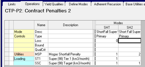
Penalties often come in tiers – where the fee changes depending on the size of the shortage. If each tranche is priced separately and the penalty increases, then you can just add another shortfall operation with a higher associated cost – as the model will always do the cheapest first. For example if the 2$ fee applies to the first 5% but is doubled after that for any further missing volume:
If the fees for other tiers are not simple multiples of the first, then define another utility code. An additional limit is used to cap the amount that can be paid for with just 1 unit of penalty.
If the higher fee for a larger shortfall applies to the whole amount, so 2$/m3 if the shortfall is 5% or less, but 4$/m3 for everything that is missing if it is greater than 5%, the model needs to understand that the more expensive option must be used on its own if needed. You don't get to use the cheaper option first. The simplest way to say that only one of a group of variables can be active at a time is to make a Type 1 Special Ordered Set. (Don’t be tempted to use a single vector with a PUP for the cost and an If… then logic on the AR panel to choose the price – that would be a step change function, not continuous, so although it would “work”, the partial would be zero almost everywhere so it is unlikely to recurse well.)
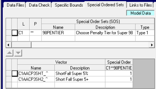
This is a very useful MIP structure - which needs a note of its own -- but in brief: give the set a name, then list the vectors that you want to include. Process unit operation matrix names consist of Location-Period-Unit-Mode. Look in the MTX or ROW output files to be sure you have the right combination and padding. If you do a comparison of the matrix files afterwards you should see the new section. The presence of the set will automatically trigger the extended optimization algorithm needed (but note that it is not supported by the HSLP optimizer - you must use XPRESS or CPLEX).
If the penalty consists of a lump sum payment, not related to the amount of short fall, but simply its existence - such as you will pay $10,000 if you deliver less than 6,000 m3, the modelling will need a binary on/off variable controlled against a threshold – a useful type of structure that I will demonstrate another time.
If your shortfall response options also include buying material on the market, then that should be included too – so that the model can balance the cost of that against the penalty conditions. Another option which is often represented in distribution models is an exchange with another supplier who has the product that you need where you are missing it, but is in need of product in another location or of another type. These can be modelled as linked purchases and sales – another useful technique that merits a separate note.
However many options you have for dealing with the issue, the optimization will choose those that maximize your profits - making the best of the situation for you. LP models push to extremes so they are quite likely to come up with solutions where many clients receive all of their requirements and some have only the minimum. LPs don’t do fair. If you have other criteria that should be applied – such as not shorting the same customer for two deliveries in a row in order to maintain good relations– then you have to translate that into a constraint on the sales so that the model understands what is acceptable. The economics are handled by the model, the business judgement still needs to come from the user.
24th December 2021.
You may also use this form to ask to be added to the distribution list so that you are notified via e-mail when new articles are posted.