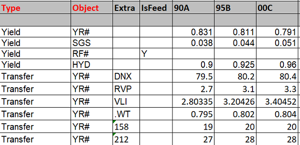
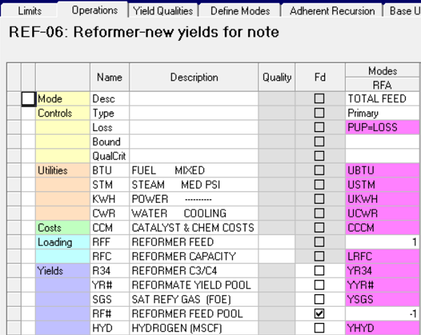
Using multiple operation modes to represent a non-linear process unit operation is very common in LP. For example, the reformate yield and qualities are non-linear functions of a reformer severity. We could use a set of modes for operations at different severities in order to represent this. Below is an example where we use three modes at 90, 95 and 100 severity to represent a reformer.
An LP can find the optimal solution that uses some combination of the modes to represent the best severity. To have this structure work properly, however, we need to ensure that only one or two adjacent modes can be active at the same time, so that a severity of 98, for example, is interpolated between the 95 and 100 data, not 90 and 100. This can be done using MIP (mixed integer programming), with a type 2 Special Ordered Set (SOS). The drawback is that in large models, MIP may cause long and unpredictable run times. In GRTMPS, we can use non-linear equations directly using Adherent Recursion. Below we’ll present a simple way to fit the above three modes representation into polynomial equations. We can then use just one mode with Adherent Recursion PUPs to model the non-linear behavior, completely avoiding MIP.
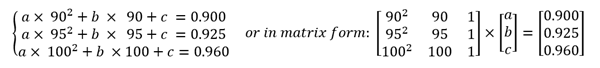
Take a look at the Hydrogen (HYD) yield, the three modes correspond to three data points : (Severity,Yield) = (90,0.900), (95,0.925) and (100,0.960). Assume that the yield (y) can be expressed as a function of the severity (x) in the polynomial form: y =ax2 +bx +c.
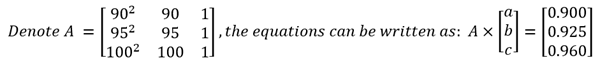
Plugging in values from the three data points, gives three simultaneous equations and three unknowns: a, b and c.
| We can find the coefficients a, b, and c by multiply the inverse of A from the left on both sides: | 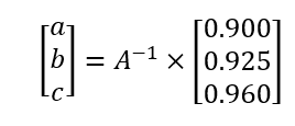 |
Excel provides array formulas for finding matrix inverse (MINVERSE) and matrix multiplication (MMULT). We can use them to easily find the polynomial coefficients a, b and c, as shown below:
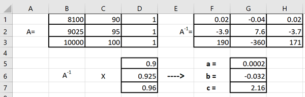
Here are the steps in the example:
- Create matrix A in cells B1:D3.
- Select cells of the same size in F1:H3.
- Type in the formula =MINVERSE($B$1:$D$3) and click Ctrl+Shift+Enter key (to indicate an array formula where the result appears in multiple cells). This gives the inverse of the matrix, A-1 in cells F1:H3.
- Create the RHS matrix in cells D5:D7.
- Select cells G5:G7. Type formula =MMULT($F$1:$H$3,D5:D7) and click Ctrl+Shift+Enter.
The coefficients a, b, and c are now in cells G5:G7. (Note: In matrix multiplication, the order matters. Make sure the cells for the inverse A matrix are given before the RHS values.)
After getting a, b and c for polynomials for all the yields, yield qualities, utilities, losses etc., we can replace the three operations with a single mode connected to these formulae via PUP codes.
The equations for the PUPs could be put in a Process Simulator Interface workbook or you can write them directly in the Adherent Recursion panel [TABLE 206.9] using Type 7 equations. Type 7 is a 6th power polynomial of the generic form Ax6 + Bx5 + Cx4 + Dx3+ Ex2 + Fx + K1. So the calculated value for a goes in E, b in F and c in K1, as shown below.
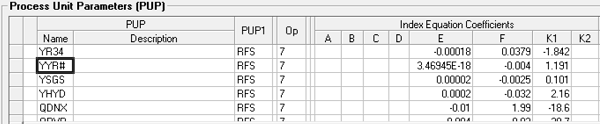
Severity, our x, is indicated under PUP1 as RFS, an operating parameter constraint controlled to the allowed range in the LP model. Where the relationship is to severity is actually linear, such as for reformate yield, code YYR#, then E is effectively zero.
The original modal representation only allowed severities in the range 90 to 100, but with a function based model, there is the possibility of extrapolating to higher and lower values - although you should plot the curve and check how far the equation looks trustworthy. Generally speaking, if we have n modes which vary with respect to the input variable, we can use this method to fit the data points into a polynomial of the (n-1) power, creating a curvilinear description of the relationship to drive the SLP optimization model.
From Richard's Desk, 22nd October 2018.
Comments and suggestions gratefully received via the usual e-mail addresses or here.
You may also use this form to ask to be added to the distribution list so that you are notified via e-mail when new articles are posted.