The purpose of software like GRTMPS is to write out a representation of your business's options as a linear programming problem, so that it can be optimized. To become an expert in this technology you need to go beyond the data entry and look at the equations that are generated. The ROW file provides one way of doing that, displaying the problem by constraints, but it is the MTX file that is actually passed to the optimizer for solving. This provides a different view of the problem, organized by variables. When studying a problem, I find it is often helpful to be able to switch between the two views – the ROW to see what variables are in a particular constraint and the MTX file to see all the places where a variable is used. To do that, you have to be able to understand the MPS format information in the MTX file. Another advantage of being able to read the MTX is that the comparison tool (see Note 34) understands the format and is able to look past differences in order and to use tolerances for identifying significant differences, while the ROW files are done just as a text comparison. To keep these files after a run, tick their boxes on the General panel of the Output node.
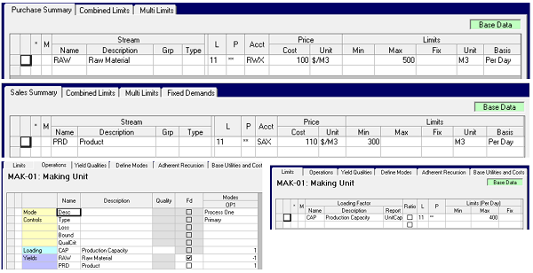
I put together a tiny little model in GRTMPS to use as an example – small enough that the whole problem can be shown. It purchases one stream, RAW, and passes it through a process unit, MAK-01, in order to convert it to PRD. This product is sold. There are limits on the purchase and sale, and a capacity constraint on the process unit.
This is exported into GRTMPS tables, in the DB$ file, as:
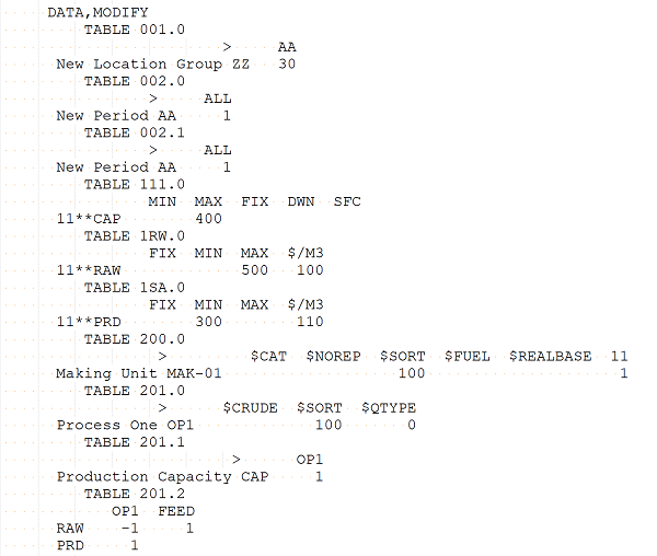
along with some other bits and pieces of basic structure, such as TABLE 911.0 for the stream list.
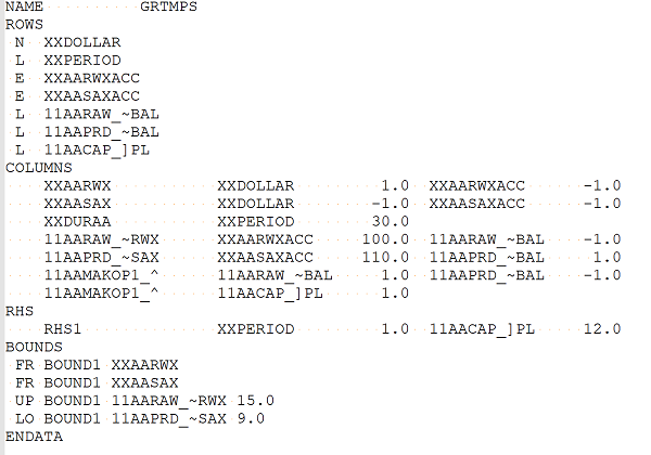
These are in turn converted into an LP problem in MPS format.
MPS format was developed by IBM for an early simplex solver code. It was designed for punch cards, one line per card, 80 characters max, each element starting in a particular column. It’s a very efficient way of writing out an LP problem and so came to be something of a standard for solver codes. MPS format has evolved a bit over the years with relaxations on the spacing and length of names, and various extensions for additional structure. Even though it has become less popular (check out the Wikipedia article), we still use it in GRTMPS as it has the great advantage of allowing us to support multiple optimizers (HSLP, XPRESS and CPLEX at present) with the same matrix generation code.
An MPS file always begins with a NAME to label the problem.
Then there is the ROWS section, to list all the constraints. Each row gives the equation sense and its name. The first row is “N” for non-constraining; this is the objective function row – usually XXDOLLAR in GRTMPS. Other rows will be “L”, “G”, or “E” for less than, greater than and equal to. GRTMPS builds the names from the model codes, to help make it clear what they represent. See Note 16: Decoding Matrix Row and Column Names.
The COLUMNS section follows next. This indicates all the intersections between the variables in the problem and the rows. All the entries for a particular column appear together. The number is the co-efficient that variable has in the named row(s). There was room on a line's punch card for two row entries.
RHS lists the Right Hand Side values for the equations. Only the non-zeros need to be given, so just two of the rows are there. (The RHS1 is a constant label – relating to an dis-used feature to put multiple constraint sets in the same problem file. Where the constraint is on a single variable, it can be done in the BOUNDS section. “FR” is for FREE – these variables are allowed to have negative values. LO is lower bound, for a minimum on a variable. Where a variable is not free and has no LO entry, then its minimum is zero. UP is upper bound for a maximum. There are other bound types for integer constraints – for example SC for semi-continuous limits.
ENDDATA lets the solver know we've finished.
Ready to translate matrix to equation? 11AARAW_~BAL, material balance on stream RAW, is an L row, with no RHS entry – that gives <=0 on the right. It has contributions from the 11AARAW_~RWX column – a purchase – and 11AAMAKOP1_^, a process vector. Combined result:
11AARAW_~RWX x -1.0 + 11AAMAKOP1_^ x 1.0 <=0.
The ROW file, by the way, doesn't write out the problem exactly as equations either, but something half-way between. The format varies a bit between optimizers. If you are running H/XPRESS, then this balance row would be expressed as:
Row = 11AARAW_~BAL Type = MAX RHS = 0.000000
11AARAW_~RWX = -1 11AAMAKOP1_^ = 1
11AARAW_~RWX = -1 11AAMAKOP1_^ = 1
Note that the numbers in the equations don’t always directly reflect the entered data. The sign convention for stream balance rows is negative for make and positive for consume. So the process unit has a positive value in the row, although RAW is the feed and has a negative in the data. (Don Alton, who retired some years ago, told me that all this was designed in an effort to minimize the number of negative signs used, as they took up one of the spaces on the punch card, restricting the number to one less significant digit.) Limits are often different as well, since data can be entered on a per day basis, but most GRTMPS models use a per period matrix – and the decimal point may have been moved to improve the scaling. So, for example, the maximum purchase of 500 m3/day of RAW becomes an upper bound of 15, when multiplied by 30 days and divided by 1000: 11AARAW_~RWX <= 15.0
Now, can you write out the rest of the equations?
A couple of final points.
- By default the MTX and ROW are the initial linear approximation. You can also keep the last ones, with the recursed entries revised to the last assumed value, by selecting them on the Output panel. For the ROW file if you choose "After Recursion" from the drop down menu, the file is not written until the final pass. There is no way to get both from the same run. The after recursion MPS formatted problem goes into a separate file. Mark "BCD Matrix After Recursion" and it will write it to a BCD file (by column description). The comparison tool can be used to compare MTX to BCD files if you want to see what has changed as a result of the recursion.
- Kirby’s Matrix Analyzer (part of the Haverly Excel Add-in) can be used to study how a particular set of equations in the final matrix has balanced out in the solution, provided that you set the option SOLTODB and kept the solution database.
From Kathy's Hotel Room, Catania, Italy
11th May2018 and updated with links to later notes on 14th March 2019.
11th May2018 and updated with links to later notes on 14th March 2019.
Comments and suggestions gratefully received via the usual e-mail addresses or here.
You may also use this form to ask to be added to the distribution list so that you are notified via e-mail when new articles are posted.