When a model doesn’t converge, one possible cause is that some of the adherent recursion PUPs don’t converge. To address this problem, one can use the adherent recursion slope damping to reduce the variations of PUPs between recursions passes to help the model to converge.
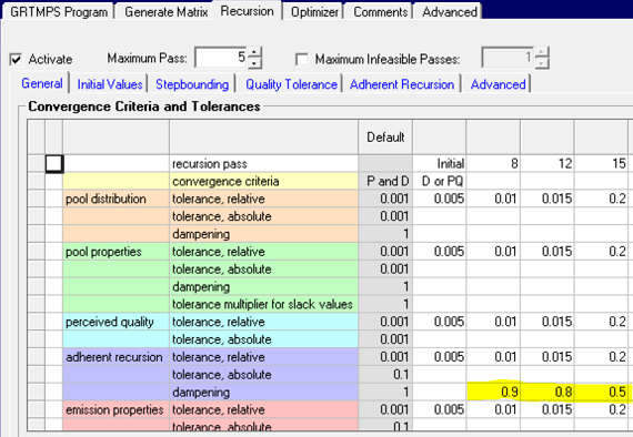
As we know, each adherent recursion PUP represents a non-linear equation in general. GRTMPS builds a linear approximation into the matrix to represent the PUP in each recursion pass. This linear approximation (base + slopes) would be updated from pass to pass. The slope damping, as its name suggests, would damp the variation of the slopes and therefore reduce the variation of the PUP to help the convergences. A slope damping factor can be set by going to the "Case | Recursion | General" tab, "Convergence Criteria and Tolerances" frame. Enter a value in the "dampening" row of the "adherent recursion" group.
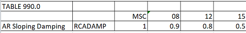
In spreadsheet models, the factor can be entered in the GRTMPS OMNI Table 990.0, in row RCADAMP column MSC or the Recursion Pass # column, as shown below.
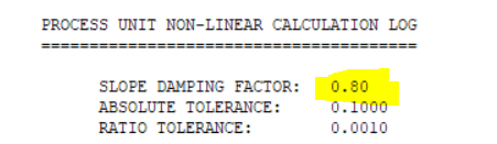
We can also find out the value of the factor in a particular pass in the output .LST file in the “PROCESS UNIT NON-LINEAR CALCULATION LOG”, as shown below.
The slope used in matrix construction will be: Smatrix = Sn * DF + Sn-1 * (1-DF)
Here DF is the sloping damping factor which usually is set to a value between 0 and 1. The default is 1. Sn is the actual slope in pass n. If the PUP equation is linear, this damping factor would have no effect because the slope is a constant.
Here DF is the sloping damping factor which usually is set to a value between 0 and 1. The default is 1. Sn is the actual slope in pass n. If the PUP equation is linear, this damping factor would have no effect because the slope is a constant.
|
The base values and slopes returned from the simulator for each non-linear process unit on each recursion pass can be found in the LST file in TABLE 2(TN).9F(LL)(PP) – where TN is the unit table ID, LL=location and PP = periods. For example, WAVWTX is the per-cent volume yield. HNT is the IBP and is currently at its maximum of 750 degrees F. If the temperature is increased by 1 degree the yield will go down by -0.3.
|
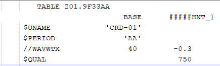 |
This information is used in the matrix for the next linear approximation, and might result in a solution that goes to the minimum value of 700 degrees, but the prediction doesn't match the actual value, indicating that the change in yield was not linear between these two points.
ITEM PLANT PERIOD UNIT TYPE ASSUMED PREDICTED ACTUAL DEVIATION NOT CONVERGED
==== ===== ====== ==== ==== ======= ========= ====== ========= =============
WAVWTX 33 AA CRD-01 YLD 40 25 30 -5 1
| We can confirm this by looking at the slope returned by the simulator on this pass. If there is no dampening, then the slope on the next pass will be -0.1. If the model returns to 750 degrees, it will predict a yield of 35%. | 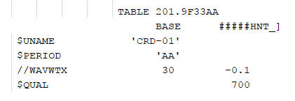 |
This oscillation between values might well continue for many more passes. But if a dampening factor is used, the slope and therefore the prediction, will change. The damped slope will take a value between the current value from the simulator (-0.1) and the one for the previous pass (-0.3), depending on the factor set.
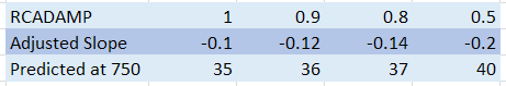
So changing the dampening factor on later passes could be enough to break any cycling. (That 0.5 gives a perfect match is just a quirk of this particular example; it is not necessarily the best value to use in general.) This technique is especially useful when the non-linear equation has peaks or valleys. That is, when the slope may change signs. As a caution, we should avoid applying this damping factor in early passes before the run stabilizes because it may distort the non-linear relationship and drive the solution to a poor value local optimal.
From Richard's and Kathy's Desks 2nd October 2017.
Comments and suggestions gratefully received via the usual e-mail addresses or here.
You may also use this form to ask to be added to the distribution list so that you are notified via e-mail when new articles are posted.